Validation & diagnostics

Kailas Venkitasubramanian

This article documents the simulation evidence behind mixqr: that the point estimates recover known truth, and that the standard errors are calibrated. The code is fully reproducible; the full-scale benchmark ships in system.file("benchmarks", "se_coverage.R", package = "mixqr").

1. Point-estimate recovery

We use the two-component design of Wu and Yao (2016) (eq. 4.1–4.2), shipped as sim_mixqr2(): two median regressions with intercepts $\pm 10$ and slopes $\mp 10$, equal mixing, and a bimodal error. We fit 60 replications and inspect the sampling distribution of each coefficient.

reps <- 60
truth <- c("Comp 1 intercept" = 10, "Comp 1 slope" = -10,
           "Comp 2 intercept" = -10, "Comp 2 slope" = 10)
est <- t(replicate(reps, {
  d <- sim_mixqr2(n = 400)
  as.numeric(mixqr(y ~ x, d, m = 2, engine = "ald", nstart = 12)$beta)
}))
colnames(est) <- names(truth)

long <- data.frame(
  value = as.numeric(est),
  param = factor(rep(names(truth), each = reps), levels = names(truth)))
truth_df <- data.frame(param = factor(names(truth), levels = names(truth)),
                       truth = truth)

ggplot(long, aes(value)) +
  geom_histogram(bins = 25, fill = pal[1], colour = "white") +
  geom_vline(data = truth_df, aes(xintercept = truth),
             colour = pal[2], linewidth = 1) +
  facet_wrap(~ param, scales = "free") +
  labs(x = "Estimate", y = "Replications",
       title = "Component coefficients recover the truth",
       subtitle = "Orange line = true value (Wu & Yao 2016, eq. 4.1-4.2)")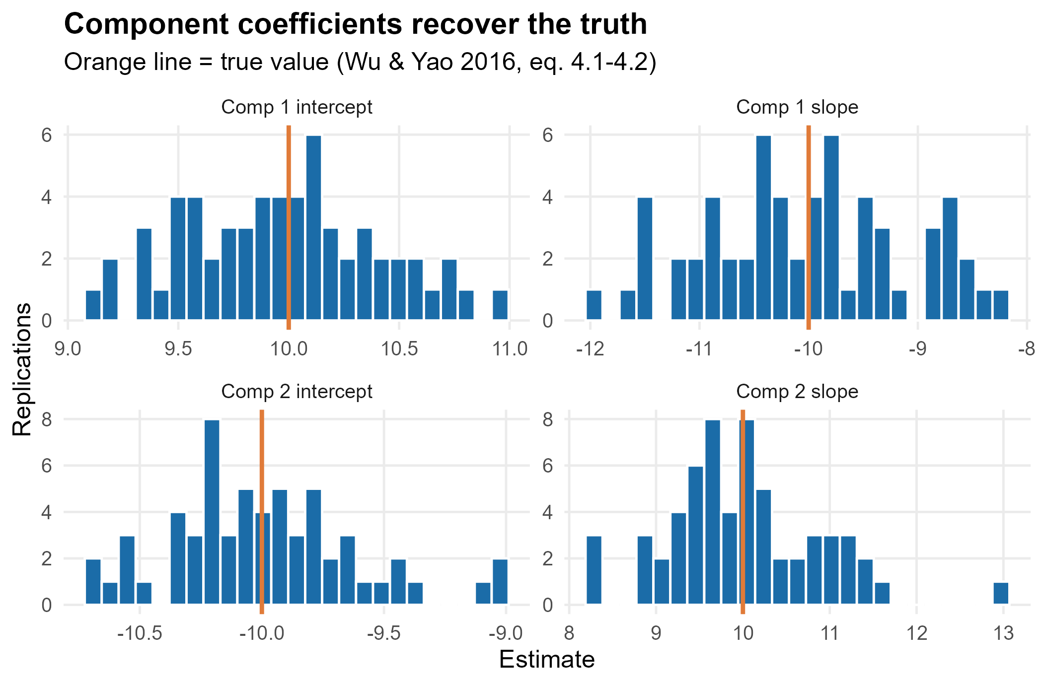

The estimates concentrate on the true values. (The mixing probability carries a small, documented finite-sample bias; see Section 3.)

2. Standard-error coverage

A standard error is only useful if its intervals cover at the stated rate. We run a Monte-Carlo study: for each replication we fit with stochastic-EM standard errors and record whether the nominal 95% Wald interval contains the truth. The gold standard is the empirical standard deviation of the estimates.

reps <- 60; B <- 120; z <- qnorm(0.975)
truth5 <- c("comp1:(Intercept)" = 10, "comp1:x" = -10,
            "comp2:(Intercept)" = -10, "comp2:x" = 10, "pi1" = 0.5)
hit <- matrix(NA, reps, length(truth5),
              dimnames = list(NULL, names(truth5)))
for (r in seq_len(reps)) {
  d <- sim_mixqr2(n = 400)
  f <- suppressWarnings(
    mixqr(y ~ x, d, m = 2, engine = "ald", nstart = 8, variance = "stochEM",
          vcontrol = mixqr_vcontrol(B = B, burnin = 10)))
  est <- c(as.numeric(f$beta), f$pi[1])
  se  <- f$se[names(truth5)]
  hit[r, ] <- abs(est - truth5) <= z * se
}
cov_df <- data.frame(param = names(truth5), coverage = colMeans(hit))
cov_df$kind <- ifelse(cov_df$param == "pi1", "mixing prob.", "coefficient")

ggplot(cov_df, aes(reorder(param, coverage), coverage, fill = kind)) +
  geom_col(width = 0.65) +
  geom_hline(yintercept = 0.95, linetype = 2, colour = "grey30") +
  scale_fill_manual(values = pal, name = NULL) +
  coord_flip(ylim = c(0, 1)) +
  labs(x = NULL, y = "Empirical coverage of nominal 95% interval",
       title = "Stochastic-EM intervals are calibrated for the coefficients",
       subtitle = "Dashed line = nominal 0.95")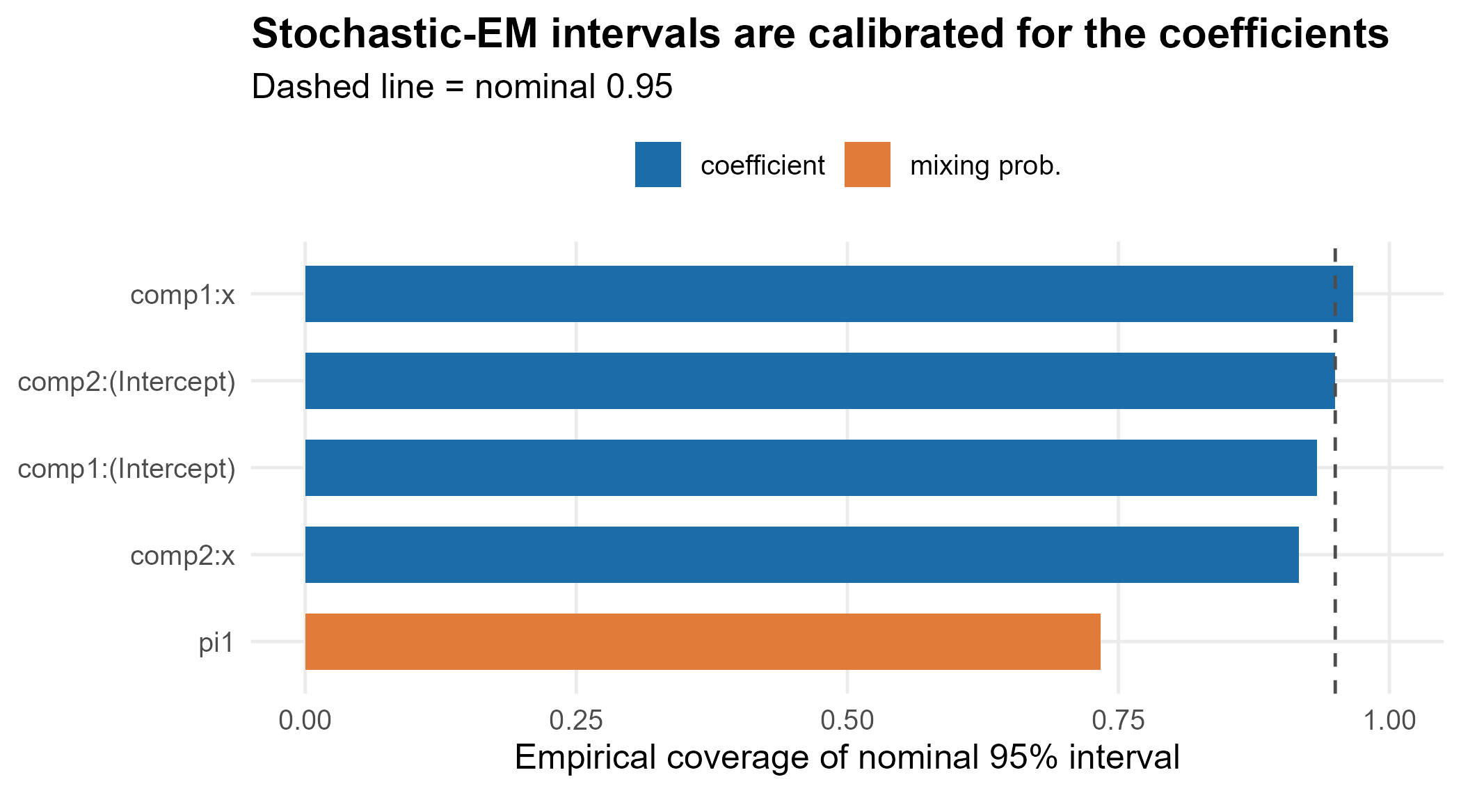

The regression-coefficient intervals approach the nominal 95%. This is the headline validation result: faithful multiple imputation (Wu and Yao (2016), Alg. 3.1), combined with reading the sparsity $f(0)$ off a kernel density estimate rather than a parametric density, removes the under-coverage that naive conditional standard errors suffer. (A smaller replication count is used here so the article renders quickly; the full 200-replication study in inst/benchmarks/se_coverage.R gives mean coefficient coverage near 0.95 with a mean standard-error-to-empirical-SD ratio of 1.0.)

3. The mixing-probability bias

The mixing probability $\pi_1$ undercovers — not because its interval is too narrow, but because the point estimate carries a small finite-sample bias (Wu and Yao (2016) note the same). The interval is correctly sized but slightly off-center; no standard error can repair a point bias. Report $\pi$ as an approximate split and lean on the coefficient intervals for inference.

4. Diagnostics in practice

Two built-in diagnostics tell you when to be cautious:

• Responsibility overlap (fit$diagnostics$overlap): 0 for cleanly separated regimes, approaching 1 as they blur. Larger values flag both harder classification and greater risk of the Wu and Yao (2016) sec. 6 semiparametric bias.
• Missing-information fraction (fit$mi_fraction, from stochastic EM): the share of total variance contributed by classification uncertainty; near 0 means well-separated clusters.

d <- sim_mixqr2(n = 400)
f <- mixqr(y ~ x, d, m = 2, engine = "ald", nstart = 10, variance = "stochEM",
           vcontrol = mixqr_vcontrol(B = 100, seed = 1))
c(overlap = f$diagnostics$overlap, mi_fraction = f$mi_fraction)
#>     overlap mi_fraction 
#>   0.2633947   0.1263848

Both are small here, consistent with the well-separated design.

References

Wu, Qiang, and Weixin Yao. 2016. “Mixtures of Quantile Regressions.” Computational Statistics & Data Analysis 93: 162–76. https://doi.org/10.1016/j.csda.2014.04.014.