Extensions: expectiles, variable selection, and non-crossing

Four capabilities on one EM platform, for applied researchers

Kailas Venkitasubramanian, University of North Carolina at Charlotte

The core of mixqr is a single EM platform: an E-step that softly assigns each observation to a latent regime, and an M-step that re-fits each regime’s regression. Version 0.2.0 keeps that platform fixed and swaps only the component loss and the coupling between fits. Because every extension inherits the same classification machinery, S3 methods, and diagnostics, they compose cleanly with the rest of the package. This article documents four of them.

Capability	Function / argument	What it changes
Expectile components	family = "expectile"	check loss → asymmetric least squares
M-quantile components	family = "mquantile"	check loss → asymmetric Huber (a robustness dial)
Component-specific selection	mixqr_pen()	each regime gets its own sparse support
Joint multi-tau, non-crossing	mixqr_nc()	one shared classification, ordered quantiles

The mechanism is an engine registry: a family or a fitting routine supplies an E-step density, an M-step solver, a log-likelihood, and a parameter count, and the driver does the rest. You can list what is registered:

list_mixqr_engines()
#> [1] "ald"       "expectile" "kdEM"      "mquantile"

1. Expectile and M-quantile families

1.1 What an expectile mixture is

A $\tau$-quantile minimises the asymmetric absolute (check) loss. An expectile at level $\theta$ minimises the asymmetric squared loss (Newey and Powell 1987): residuals above the fit are weighted $\theta$ and those below $1-\theta$. Swapping absolute for squared has two consequences. The objective becomes strictly convex and smooth, so each component has a unique solution found by a fast iteratively-reweighted least squares (no linear program); and the fitted expectile, like a mean, responds to the magnitude of every residual, which makes it more efficient under light-tailed errors but sensitive to gross outliers. An expectile mixture simply fits a $\theta$-expectile regression inside each latent regime.

Use the family argument. We work with the Dutch nlschools data (Venables and Ripley (2002); language-test scores of 2287 eighth-graders), standardising SES and asking whether the SES–achievement gradient splits into two regimes.

data(nlschools, package = "MASS")
nl <- nlschools
nl$SES <- as.numeric(scale(nl$SES))

fit_e <- mixqr(lang ~ SES, data = nl, tau = 0.5, m = 2,
               family = "expectile", nstart = 15)
round(fit_e$beta, 3)
#>               [,1]   [,2]
#> (Intercept) 48.100 37.288
#> SES          1.378  3.716

c(family = fit_e$family, engine = fit_e$engine)
#>      family      engine 
#> "expectile" "expectile"

Two regimes emerge: a low-baseline, steep-gradient regime and a higher-baseline, shallower one. The fitted expectile coefficients are read exactly like quantile coefficients, but they summarise a smoothed asymmetric centre rather than a strict quantile.

1.2 When to prefer an expectile (efficiency vs robustness)

The trade is efficiency for robustness. Expectiles use every residual’s magnitude, so under clean, light-tailed data they are more stable from sample to sample; but a few gross outliers can drag them far, exactly as they drag a mean. A direct demonstration: fit each family on a clean two-regime design, then contaminate 2% of the responses with large positive shifts and re-fit.

set.seed(11)
clean <- sim_mixqr2(n = 400)                 # 2-regime median design
slopes <- function(d, fam)
  sort(mixqr(y ~ x, d, tau = 0.5, m = 2, family = fam, nstart = 12)$beta[2, ])

dirty <- clean
hit <- sample(nrow(dirty), 8)                # 2% gross outliers
dirty$y[hit] <- dirty$y[hit] + 80

shift <- sapply(c("quantile", "mquantile", "expectile"), function(f)
  sum(abs(slopes(dirty, f) - slopes(clean, f))))
round(shift, 2)
#>  quantile mquantile expectile 
#>      1.54      1.28     16.40

sh <- data.frame(family = names(shift), shift = as.numeric(shift))
ggplot(sh, aes(reorder(family, shift), shift, fill = family)) +
  geom_col(width = 0.6) +
  scale_fill_manual(values = pal, guide = "none") +
  coord_flip() +
  labs(x = NULL, y = "Total slope shift under 2% contamination",
       title = "Robustness is the price of expectile efficiency",
       subtitle = "Quantile and M-quantile barely move; the expectile collapses")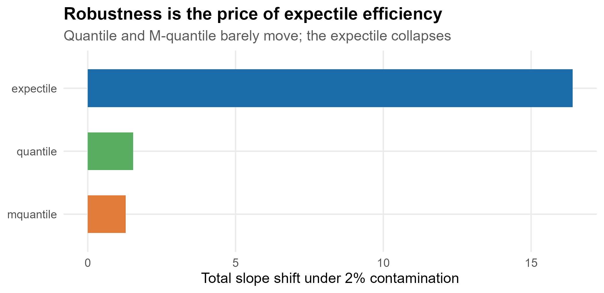

The check-loss (quantile) and asymmetric-Huber (M-quantile) slopes barely move, while the expectile slopes are pulled apart by the eight contaminating points. Prefer expectiles when the errors are well-behaved and you want the extra efficiency and smoothness (or you want a quantity that, like a mean, integrates to the conditional mean over $\theta$); prefer quantiles when robustness to the tails is the whole point, which in most applied quantile work it is.

1.3 The crossing-free-in-theta property

One structural advantage comes for free. The fitted $\theta$-expectile is monotone in $\theta$by construction (a property of asymmetric least squares), so expectile lines fitted at a grid of asymmetry levels cannot cross within a component – no constraint machinery, no rearrangement. Quantile fits enjoy no such guarantee in finite samples (that is what Section 3 repairs). We verify it directly: fit at a grid of $\theta$ and check the per-component curves over the SES range.

thetas <- c(0.1, 0.25, 0.5, 0.75, 0.9)
fits_e <- lapply(thetas, function(th)
  mixqr(lang ~ SES, nl, tau = th, m = 2, family = "expectile", nstart = 12))

xs <- seq(-2, 2, length.out = 60)
crossings <- 0
for (j in 1:2) {
  Q <- sapply(fits_e, function(f) cbind(1, xs) %*% f$beta[, j])
  crossings <- crossings + sum(apply(Q, 1, function(r) sum(diff(r) < -1e-8)))
}
crossings
#> [1] 0

band <- do.call(rbind, lapply(seq_along(thetas), function(i) {
  f <- fits_e[[i]]
  do.call(rbind, lapply(1:2, function(j)
    data.frame(SES = xs, lang = as.numeric(cbind(1, xs) %*% f$beta[, j]),
               component = paste("Component", j), theta = thetas[i])))
}))

ggplot(band, aes(SES, lang, group = interaction(component, theta),
                 colour = component, alpha = theta)) +
  geom_line(linewidth = 1) +
  scale_colour_manual(values = pal2, name = NULL) +
  scale_alpha_continuous(range = c(0.35, 1), name = expression(theta)) +
  labs(x = "Family SES (standardised)", y = "Language score",
       title = "Expectile curves never cross within a component",
       subtitle = "Five theta levels per regime; monotone in theta by construction")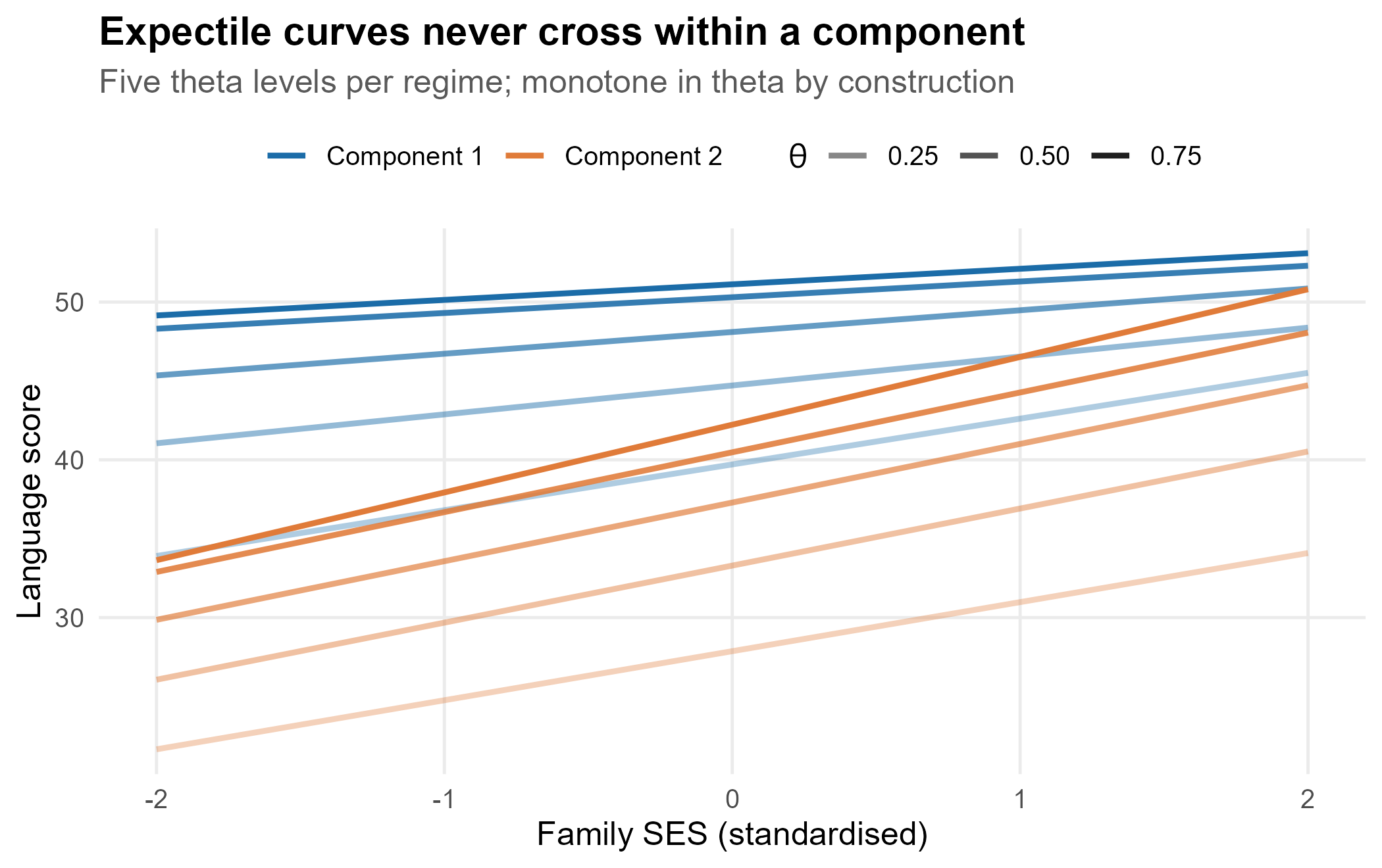

Zero crossings across the design. The expectile family is the natural choice when you want several asymmetry levels and a built-in non-crossing guarantee.

1.4 The M-quantile dial

The M-quantile (Breckling and Chambers 1988) replaces the squared loss with an asymmetric Huber loss: quadratic near zero, linear beyond a cutoff $c\cdot\sigma$. The cutoff is a dial. As $c\to 0$ the M-quantile approaches the quantile (fully robust, linear loss); as $c\to\infty$ it approaches the expectile (fully efficient, quadratic loss). The default $c = 1.345$ is Huber’s 95%-efficiency constant. Set it through control$mq_c and watch the slopes slide between the two endpoints.

dial <- function(cc) {
  ct <- mixqr_control(); ct$mq_c <- cc
  f <- mixqr(lang ~ SES, nl, tau = 0.5, m = 2, family = "mquantile",
             nstart = 12, control = ct)
  sort(f$beta[2, ], decreasing = TRUE)
}
endpoints <- list(
  quantile  = sort(mixqr(lang ~ SES, nl, tau = .5, m = 2,
                         family = "quantile",  nstart = 12)$beta[2, ], TRUE),
  expectile = sort(mixqr(lang ~ SES, nl, tau = .5, m = 2,
                         family = "expectile", nstart = 12)$beta[2, ], TRUE))

tab <- rbind(`mq_c=0.5`   = dial(0.5),
             `mq_c=1.345` = dial(1.345),
             `mq_c=5`     = dial(5))
round(rbind(quantile = endpoints$quantile, tab,
            expectile = endpoints$expectile), 3)
#>             [,1]  [,2]
#> quantile   4.363 2.182
#> mq_c=0.5   4.083 2.375
#> mq_c=1.345 3.532 2.151
#> mq_c=5     3.226 1.953
#> expectile  3.716 1.378

The slopes for the steeper component (first column) move monotonically from the quantile value at a small cutoff toward the expectile value at a large one: the M-quantile genuinely interpolates between robust and efficient. Use a small cutoff when a few outliers should not dominate, a large one when efficiency matters and the data are clean.

2. Component-specific penalized selection

2.1 Motivation: each regime its own sparse support

In a high-dimensional regression you select variables once. In a mixture of regressions, the right support can differ by regime: a covariate that drives the outcome in one latent cluster may be irrelevant in another. mixqr_pen() gives each component its own penalised check-loss M-step – a SCAD / adaptive-LASSO / LASSO / MCP penalty on the slopes (the intercept is never penalised), the quantile analogue of Khalili and Chen (2007). The penalty strength is tuned by a mixture BIC over a path, and components whose mixing weight vanishes are pruned.

2.2 A worked example

We simulate ten candidate covariates and a two-regime outcome in which the regimes depend on disjoint covariate sets: regime A on x1, x2, regime B on x4, x5, with x3, x6–x10 pure noise. A good selector should recover the two supports separately and zero the noise.

set.seed(7)
n <- 300; p <- 10
X <- matrix(rnorm(n * p), n); colnames(X) <- paste0("x", 1:p)
z <- rbinom(n, 1, 0.5)
y <- ifelse(z == 0, 1 + 2 * X[, 1] - 1.5 * X[, 2],
                   -1 + 2 * X[, 4] + 1.5 * X[, 5]) + rnorm(n)
dat <- data.frame(y = y, X)

fit_pen <- mixqr_pen(y ~ ., data = dat, tau = 0.5, m = 2, penalty = "SCAD",
                     nstart = 12, control = mixqr_control(seed = 1))
selectedVars(fit_pen)
#> $comp1
#> [1] "x4" "x5"
#> 
#> $comp2
#> [1] "x1" "x2"

selectedVars() recovers exactly the two disjoint supports – one component picks {x1, x2}, the other {x4, x5}, and every noise covariate is dropped. The full coefficient matrix confirms the sparsity:

round(fit_pen$beta, 2)
#>              [,1]  [,2]
#> (Intercept) -0.94  1.07
#> x1           0.00  1.84
#> x2           0.00 -1.58
#> x3           0.00  0.00
#> x4           2.14  0.00
#> x5           1.37  0.00
#> x6           0.00  0.00
#> x7           0.00  0.00
#> x8           0.00  0.00
#> x9           0.00  0.00
#> x10          0.00  0.00

2.3 The BIC path

Tuning is by mixture BIC over a $\lambda$ path that runs from a value zeroing every slope down to near-zero penalty. The chosen model is the BIC minimum; the path itself is informative.

path <- fit_pen$selection$path
best <- fit_pen$selection$lambda

ggplot(path, aes(lambda, bic)) +
  geom_line(colour = pal[1]) +
  geom_point(size = 1.6, colour = pal[1]) +
  geom_vline(xintercept = best, linetype = 2, colour = pal[2]) +
  scale_x_log10() +
  labs(x = expression(lambda~"(log scale)"), y = "Mixture BIC",
       title = "Selecting the penalty by mixture BIC",
       subtitle = sprintf("Chosen lambda = %.3f (orange); pruned to %d components",
                          best, fit_pen$m))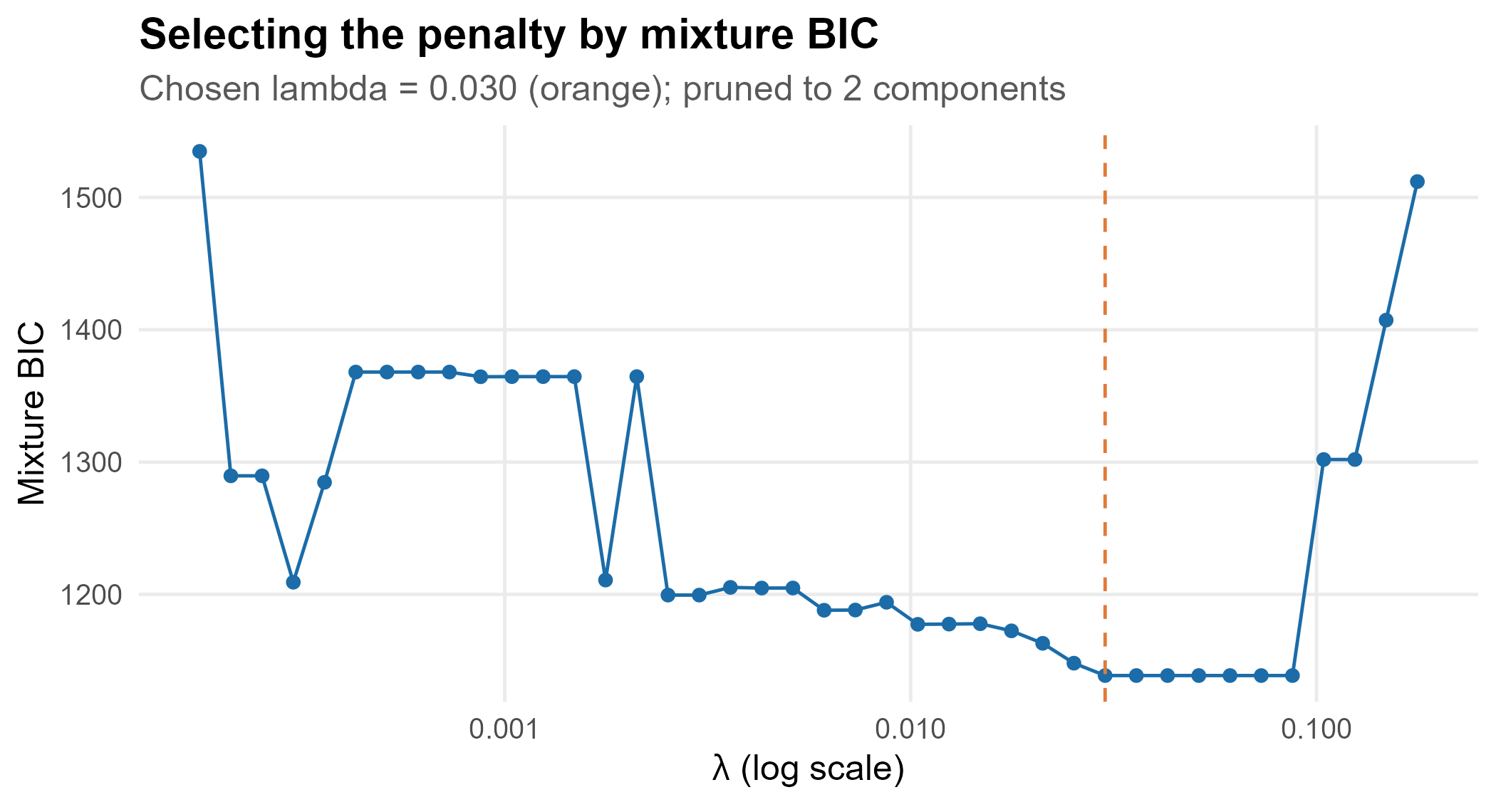

The BIC drops sharply as the penalty relaxes enough to admit the four true signals, then flattens; the minimum sits at lambda = 0.03. Heavy penalties (left) starve the model of real predictors; negligible penalties (right) re-admit noise and pay for it in the complexity term. Read the selected support, not just the curve: here it is the two clean, component-specific sets above.

3. Joint multi-tau: shared classification and non-crossing

Fitting several quantile levels separately (as in the Tutorial, Section 9) leaves two problems that Wu and Yao (2016) explicitly place out of scope:

1. Cross-level classification ambiguity. Each level estimates its own latent labels, so an observation can be “regime A at the median, regime B at the upper tail” – incoherent.
2. Within-component crossing. A component’s separately fitted quantile lines can cross in finite samples, implying a lower quantile above a higher one.

mixqr_nc() fits a vector of tau jointly: a single coupled E-step pools the per-level likelihoods so one classification is shared across all levels, and the fitted quantiles within each component are made non-crossing by monotone rearrangement (Chernozhukov, Fernández-Val, and Galichon 2010).

3.1 Demonstrating, and removing, crossing

sim_mixqr_cross() builds a design where one component is well-behaved and the other is near-flat and strongly heteroscedastic, so its separate per-tau fits cross in a small sample. We fit twice: with crossing left in (noncrossing = "none", for diagnosis) and with it repaired ("rearrange", the default).

d <- sim_mixqr_cross(n = 160, seed = 1)
taus <- c(0.1, 0.25, 0.5, 0.75, 0.9)

fit_none <- mixqr_nc(y ~ x, data = d, m = 2, tau = taus,
                     noncrossing = "none", control = mixqr_control(seed = 1))
fit_nc   <- mixqr_nc(y ~ x, data = d, m = 2, tau = taus,
                     noncrossing = "rearrange", control = mixqr_control(seed = 1))

rbind(none      = unlist(fit_none$crossing[c("raw", "after")]),
      rearrange = unlist(fit_nc$crossing[c("raw", "after")]))
#>           raw after
#> none        4     4
#> rearrange   4     0

Both fits exhibit the same 4 raw crossings on the training design; rearrangement drives the count to 0, while leaving it in keeps all 4. The diagnostic is measured on the data, not assumed.

curves <- function(fit, label) {
  P <- predict(fit)                                   # n x m x L
  xv <- fit$x[, 2]; ord <- order(xv)
  do.call(rbind, lapply(1:dim(P)[2], function(j)
    do.call(rbind, lapply(seq_along(taus), function(l)
      data.frame(x = xv[ord], q = P[ord, j, l],
                 component = paste("Component", j),
                 tau = taus[l], panel = label)))))
}
both <- rbind(curves(fit_none, "noncrossing = none"),
              curves(fit_nc,   "noncrossing = rearrange"))

ggplot(both, aes(x, q, colour = component, group = interaction(component, tau))) +
  geom_line(linewidth = 0.8) +
  facet_wrap(~ panel) +
  scale_colour_manual(values = pal2, name = NULL) +
  labs(x = "x", y = "Fitted quantile",
       title = "Monotone rearrangement removes within-component crossing",
       subtitle = "Left: five tau curves can cross. Right: ordered, by construction")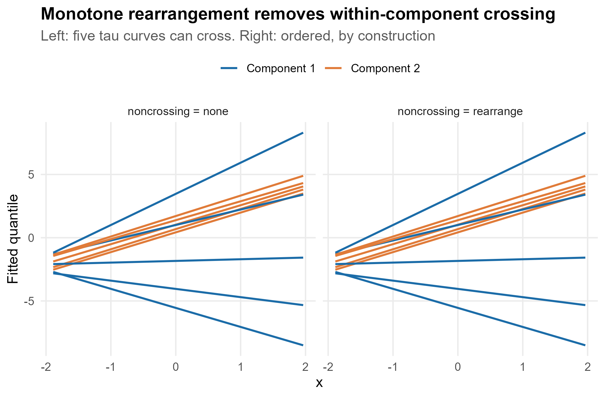

3.2 Shared classification and ordered prediction

Because one classification is shared, every observation has a single regime label that holds across all five levels – the coherence the separate fits lack.

table(component = fit_nc$classification)
#> component
#>   1   2 
#>  50 110
fit_nc$mix_prop
#> [1] 0.3580266 0.6419734

predict() returns an $[n, m, L]$ array whose last axis is the (rearranged) quantile grid, so each component’s predicted quantiles are non-decreasing in tau by construction:

P <- predict(fit_nc)
dim(P)
#> [1] 160   2   5
round(P[1, 1, ], 3)                 # observation 1, component 1, across tau
#>  tau0.1 tau0.25  tau0.5 tau0.75  tau0.9 
#>  -4.253  -3.486  -1.950  -0.049   1.346
all(diff(P[1, 1, ]) >= -1e-8)       # ordered?
#> [1] TRUE

The fit carries a print() and summary() method, and a plot() method that overlays the non-crossing curves:

fit_nc
#> Joint multi-tau mixture of quantile regressions (mixqr_nc)
#>   m = 2 components, tau = {0.1, 0.25, 0.5, 0.75, 0.9}
#>   classification coupling: pool | non-crossing: rearrange
#>   mixing proportions: 0.358, 0.642
#>   within-component crossings: 4 (raw) -> 0 (after)

plot(fit_nc)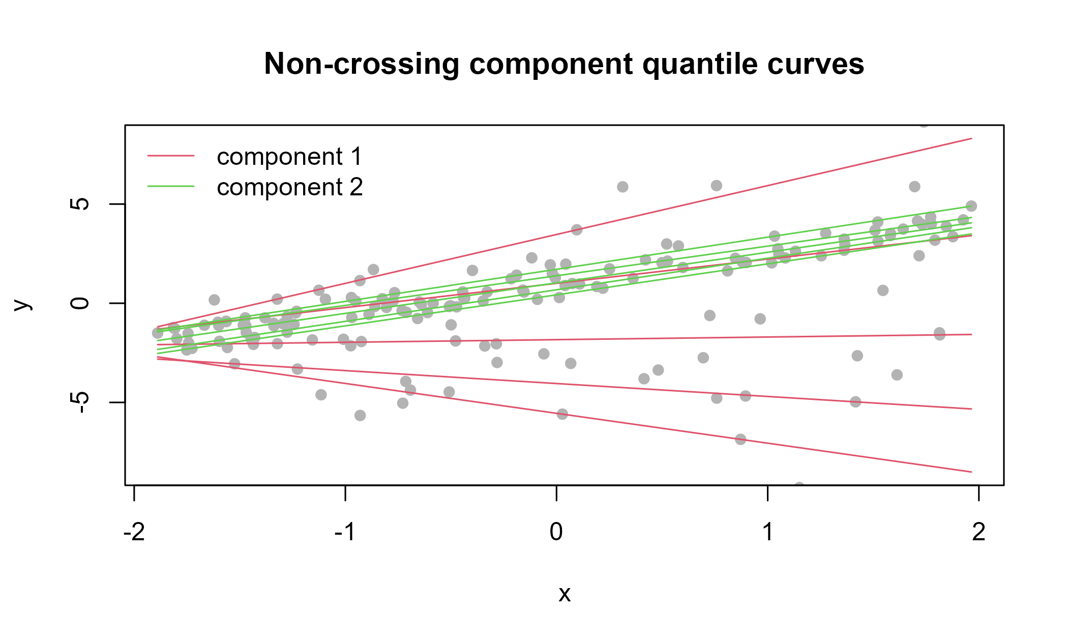

4. Practical guidance: how the capabilities relate

• Non-crossing, two ways. Expectiles (Section 1.3) are non-crossing in the asymmetry level for free, because the loss is smooth and the solution monotone. Quantiles get there by constraint – the rearrangement inside mixqr_nc() (Section 3). Choose expectiles when their interpretation suits you and the data are clean; choose constrained quantiles when you need genuine quantiles with guaranteed ordering across tau.
• Robustness is a dial. The M-quantile (Section 1.4) sits between the fully robust quantile and the fully efficient expectile; reach for it when you want some of each. The contamination experiment (Section 1.2) is the honest summary: efficiency and robustness trade off, and the family argument is how you pick your point on that curve.
• Selection composes. mixqr_pen() selects variables per component, so a regime can have its own parsimonious story. It uses the check loss; combining it with the smoother families is a natural next step but is not part of this release.
• One platform. All four ride the same EM driver, S3 methods, and overlap diagnostic. The family argument and mixqr_pen() / mixqr_nc() are different doors into the same house: whatever you learned about classifying observations, reading coefficients, and checking separation in the Tutorial carries over unchanged.

References

Breckling, Jens, and Ray Chambers. 1988. “M-Quantiles.” Biometrika 75 (4): 761–71.

Chernozhukov, Victor, Iván Fernández-Val, and Alfred Galichon. 2010. “Quantile and Probability Curves Without Crossing.” Econometrica 78 (3): 1093–1125.

Khalili, Abbas, and Jiahua Chen. 2007. “Variable Selection in Finite Mixture of Regression Models.” Journal of the American Statistical Association 102 (479): 1025–38.

Newey, Whitney K., and James L. Powell. 1987. “Asymmetric Least Squares Estimation and Testing.” Econometrica 55 (4): 819–47.

Venables, W. N., and B. D. Ripley. 2002. Modern Applied Statistics with s. Fourth. New York: Springer.

Wu, Qiang, and Weixin Yao. 2016. “Mixtures of Quantile Regressions.” Computational Statistics & Data Analysis 93: 162–76. https://doi.org/10.1016/j.csda.2014.04.014.