Quantile-function mixtures and distributional synthetic controls

Kailas Venkitasubramanian, University of North Carolina at Charlotte

qfmix approximates a quantile function by a weighted mixture of quantile basis functions and estimates the weights by matching L-moments – a convex problem – following Alvarez & Orestes (2024). It then provides confidence bands by a numerical bootstrap, and a distributional synthetic-control wrapper.

library(qfmix)
library(ggplot2)

Fitting a quantile-function mixture

We simulate from a known Pareto-quantile mixture and recover it. The individual weights of a correlated basis are weakly identified, but the fitted quantile function tracks the truth closely.

lambda <- c(1, 0.6, 0.3)
x <- sim_qmix(n = 4000, basis = "pareto", p = 3, lambda = lambda)
fit <- qfmix(x, basis = "pareto", p = 3, L = 5, constraint = "nonneg")
fit
#> Sieve quantile-function mixture (qfmix)
#>   basis = pareto   p = 3   L = 5   constraint = nonneg
#>   trim = [0, 1]   GMLM objective = -0.3777
#> 
#> Weights (lambda):
#>     b1     b2     b3 
#> 1.0751 0.2174 0.6483

u <- ppoints(200)
df <- data.frame(
  u = u,
  truth = as.numeric(qfmix_basis("pareto", 3)$eval(u) %*% lambda),
  fitted = predict(fit, u))

ggplot(df, aes(u)) +
  geom_line(aes(y = truth, colour = "truth"), linewidth = 1.2) +
  geom_line(aes(y = fitted, colour = "fitted"), linewidth = 1, linetype = 2) +
  scale_colour_manual(values = c(truth = "grey40", fitted = "#1b6ca8"),
                      name = NULL) +
  labs(x = "u", y = "quantile",
       title = "Recovered mixture quantile function") +
  theme_minimal(base_size = 12) + theme(legend.position = "top")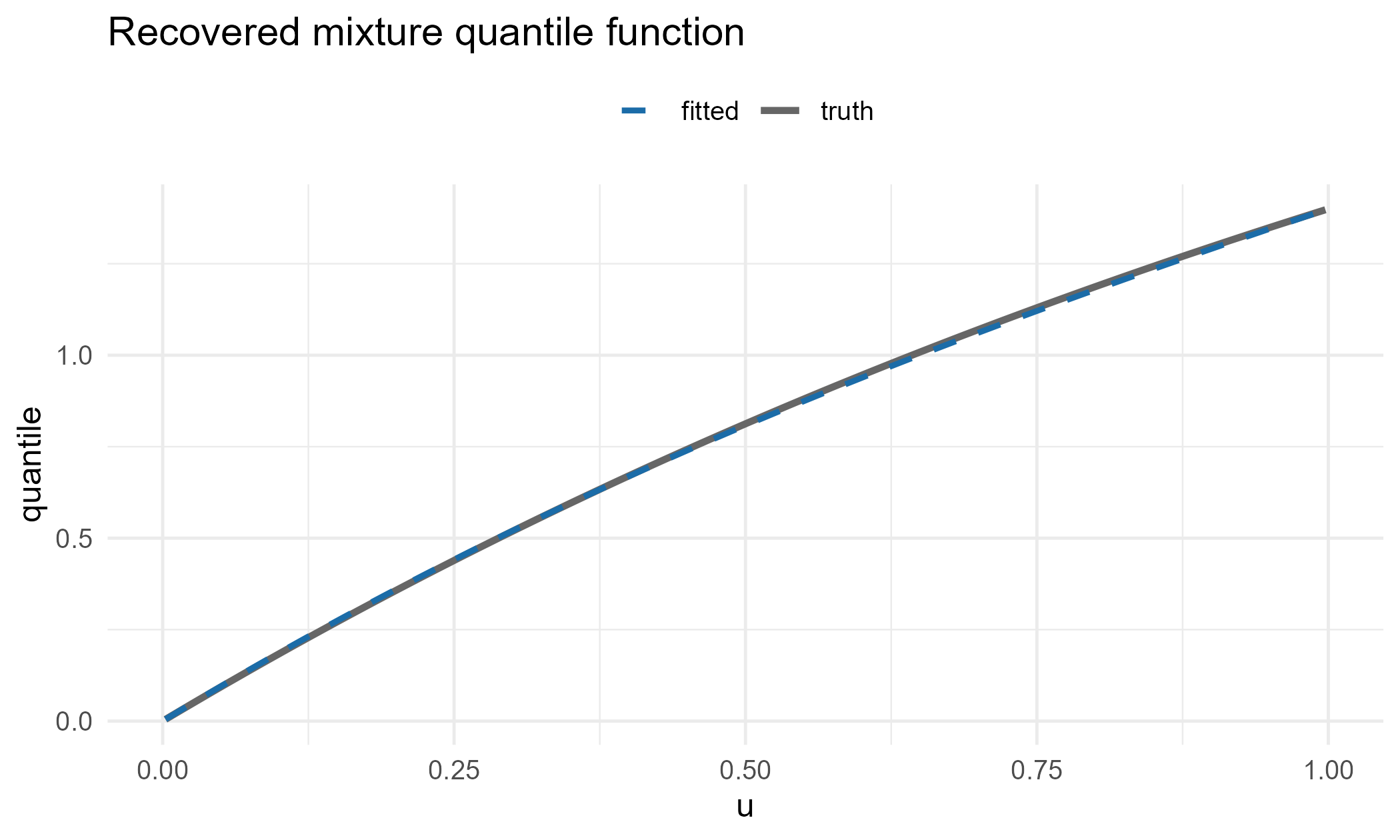

Inference: the numerical bootstrap

Inference is a simulation from the strong-approximation limit of the quantile process, not a resampling bootstrap. qfmix_boot() returns a pointwise band for the quantile function.

bt <- qfmix_boot(fit, S = 500, target = "quantile", u = u)

ggplot(data.frame(u = u, est = bt$estimate, lo = bt$lower, hi = bt$upper),
       aes(u, est)) +
  geom_ribbon(aes(ymin = lo, ymax = hi), fill = "#1b6ca8", alpha = 0.2) +
  geom_line(linewidth = 1.1, colour = "#1b6ca8") +
  labs(x = "u", y = "quantile",
       title = "Mixture quantile with 95% numerical-bootstrap band") +
  theme_minimal(base_size = 12)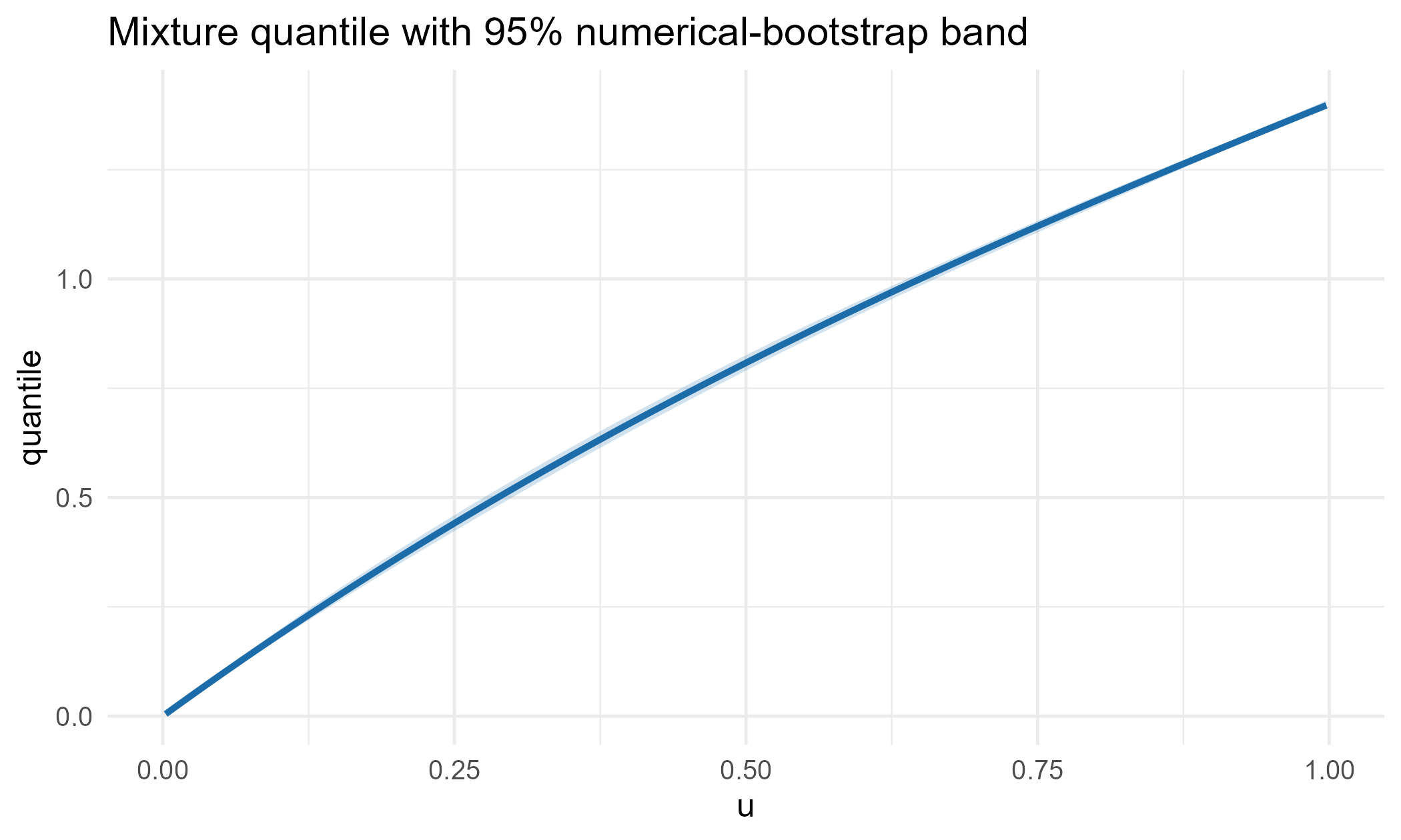

Distributional synthetic controls

The flagship application: build a counterfactual distribution for a treated unit as a mixture of control units’ distributions, with confidence bands.

# synthetic panel: four control units and a treated unit that, pre-treatment,
# resembles a blend of the controls; a shift is added post-treatment
mk <- function(id, year, mu, sd = 1) data.frame(
  unit = id, year = year, y = rnorm(200, mu, sd))
controls <- Map(function(j, mu) do.call(rbind, lapply(2016:2020, mk, id = j, mu = mu)),
                paste0("c", 1:4), c(0, 2, 4, 6))
treated <- do.call(rbind, lapply(2016:2020, function(t)
  mk("treated", t, mu = 2 + ifelse(t > 2018, 1.5, 0))))   # +1.5 shift from 2019
panel <- rbind(do.call(rbind, controls), treated)

fit_dsc <- dsc(panel, "unit", "year", "y", treated = "treated", t0 = 2018,
               constraint = "ridge", M = 1, S = 300,
               band = "uniform", bias_aware = TRUE)
fit_dsc
#> Distributional synthetic control (qfmix_dsc)
#>   treated = treated   t0 = 2018   #controls = 4   constraint = ridge
#>   pre-treatment quantile RMSE = 0.07462
#>   bands: uniform, bias-aware
#>   post periods: 2019, 2020
summary(fit_dsc)
#> Distributional treatment effects (observed - counterfactual quantile):
#> 
#> period 2019:
#>  percentile effect
#>          10  1.704
#>          25  1.686
#>          50  1.489
#>          75  1.432
#>          90  1.268
#> 
#> period 2020:
#>  percentile effect
#>          10  1.708
#>          25  1.527
#>          50  1.431
#>          75  1.480
#>          90  1.359

The distributional treatment effect at a post-period, with its band:

pr <- fit_dsc$periods[["2019"]]
ggplot(data.frame(u = pr$u, eff = pr$effect,
                  lo = pr$band$eff_lower, hi = pr$band$eff_upper),
       aes(u, eff)) +
  geom_ribbon(aes(ymin = lo, ymax = hi), fill = "#e07b39", alpha = 0.2) +
  geom_line(linewidth = 1.1, colour = "#e07b39") +
  geom_hline(yintercept = 0, linetype = 3) +
  labs(x = "u", y = "observed - counterfactual quantile",
       title = "Distributional treatment effect, 2019",
       subtitle = "A roughly uniform upward shift, as simulated") +
  theme_minimal(base_size = 12)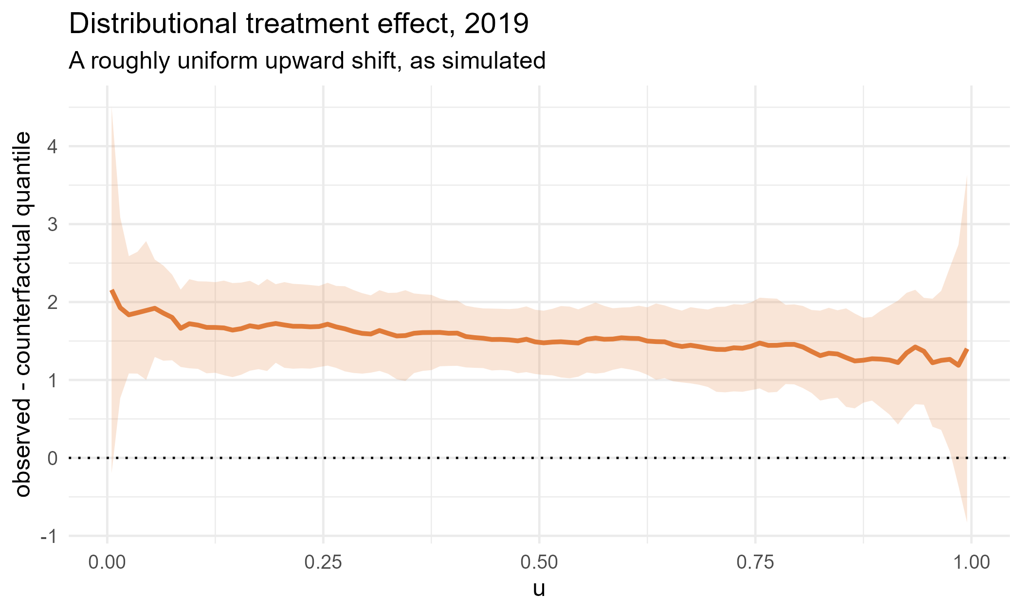

The effect is positive across the distribution, recovering the simulated +1.5 shift, and the band excludes zero. We used band = "uniform" for a simultaneous band over the whole quantile grid and bias_aware = TRUE, which widens the band by the pre-treatment approximation error where the control mixture cannot represent the treated distribution. In Monte-Carlo checks these two together lift counterfactual coverage from about 0.69 (variance-only, pointwise) to roughly the nominal 0.95 – the formal inference distributional synthetic controls have lacked, built on the strong-approximation argument of Alvarez & Orestes (2024) rather than a resampling proxy. Two refinements remain (see ?dsc): the control-sampling variance and the exact ridge-ball anti-concentration constant.

References

• Alvarez, L. A. F. & Orestes, V. M. (2024). Quantile Mixture Models: Estimation and Inference. Working paper.
• Gunsilius, F. F. (2023). Distributional synthetic controls. Econometrica 91, 1105–1117.
• Hosking, J. R. M. (1990). L-moments. JRSS-B 52, 105–124.