A Primer on Quantile-Function Mixtures and Distributional Synthetic Controls
Kailas Venkitasubramanian, University of North Carolina at Charlotte
Source:vignettes/qfmix-primer.Rmd
qfmix-primer.RmdThis primer is for applied researchers who care about effects on a whole distribution, not just its average: a policy that lifts the bottom of the wage distribution while leaving the top untouched, a shock that fattens the lower tail, a programme that compresses inequality. It assumes no background in L-moments or synthetic controls. By the end you will be able to approximate a distribution, attach confidence bands, and run a distributional synthetic control with calibrated inference, then read and report all of it.
library(qfmix)
library(ggplot2)

theme_set(theme_minimal(base_size = 12))
blue <- "#1b6ca8"; orange <- "#e07b39"
1. The question
Mean-based methods answer “did the average move?” Many policy
questions are distributional: a minimum wage should raise low
wages and barely touch high ones; a transfer programme should compress
the spread. To see those effects you need the counterfactual
quantile function – what the whole distribution
would have been without the intervention – and a way to say
which differences are real. That is what qfmix
provides.
2. Two ideas in one page
Mixing quantile functions. A quantile function maps
a probability to the value below which a fraction of the outcome falls
(the median is ). qfmix approximates a target quantile
function as a weighted combination of basis quantile functions,
where the are known (polynomials, Pareto/extreme-value shapes, or – for
synthetic controls – the empirical quantile functions of control units)
(Alvarez and Orestes 2024).
Matching L-moments. The weights are chosen so the
mixture’s L-moments match the sample’s. L-moments are
averages of order statistics – the first is the mean, the second a
measure of spread, the third of skewness (Hosking
1990) – and they are projections of the quantile function onto an
orthonormal polynomial basis. Matching them is a convex
quadratic program, so estimation is fast and has a unique
best-fitting quantile function. The weights can be left free, kept
non-negative, put on a budget (ridge), or forced onto the
probability simplex.
Inference uses a numerical bootstrap – not resampling, but a simulation from the known large-sample law of the quantile process (Csörgő and Révész 1978; Hong and Li 2020).
3. Warm-up: approximating one distribution
Wages are right-skewed. We draw a log-normal sample and approximate its quantile function with a shifted-Legendre basis.
wages <- rlnorm(800, meanlog = 3, sdlog = 0.5)         # a skewed wage sample
fit1 <- qfmix(wages, basis = "legendre", p = 5)
fit1
#> Sieve quantile-function mixture (qfmix)
#>   basis = legendre   p = 5   L = 7   constraint = unconstrained
#>   trim = [0, 1]   GMLM objective = -335.9
#>
#> Weights (lambda):
#>      b1      b2      b3      b4      b5
#> 22.8267 11.0892  3.7174  3.2157  1.9138
predict() returns the fitted quantiles; we overlay them
on the empirical ones.
u <- ppoints(100)
df <- data.frame(u = u,
                 empirical = quantile(wages, u, names = FALSE),
                 fitted = predict(fit1, u))
ggplot(df, aes(u)) +
  geom_line(aes(y = empirical, colour = "empirical"), linewidth = 1.3) +
  geom_line(aes(y = fitted, colour = "fitted"), linewidth = 1, linetype = 2) +
  scale_colour_manual(values = c(empirical = "grey45", fitted = blue), name = NULL) +
  labs(x = "u (probability)", y = "wage",
       title = "A five-term mixture captures a skewed distribution") +
  theme(legend.position = "top")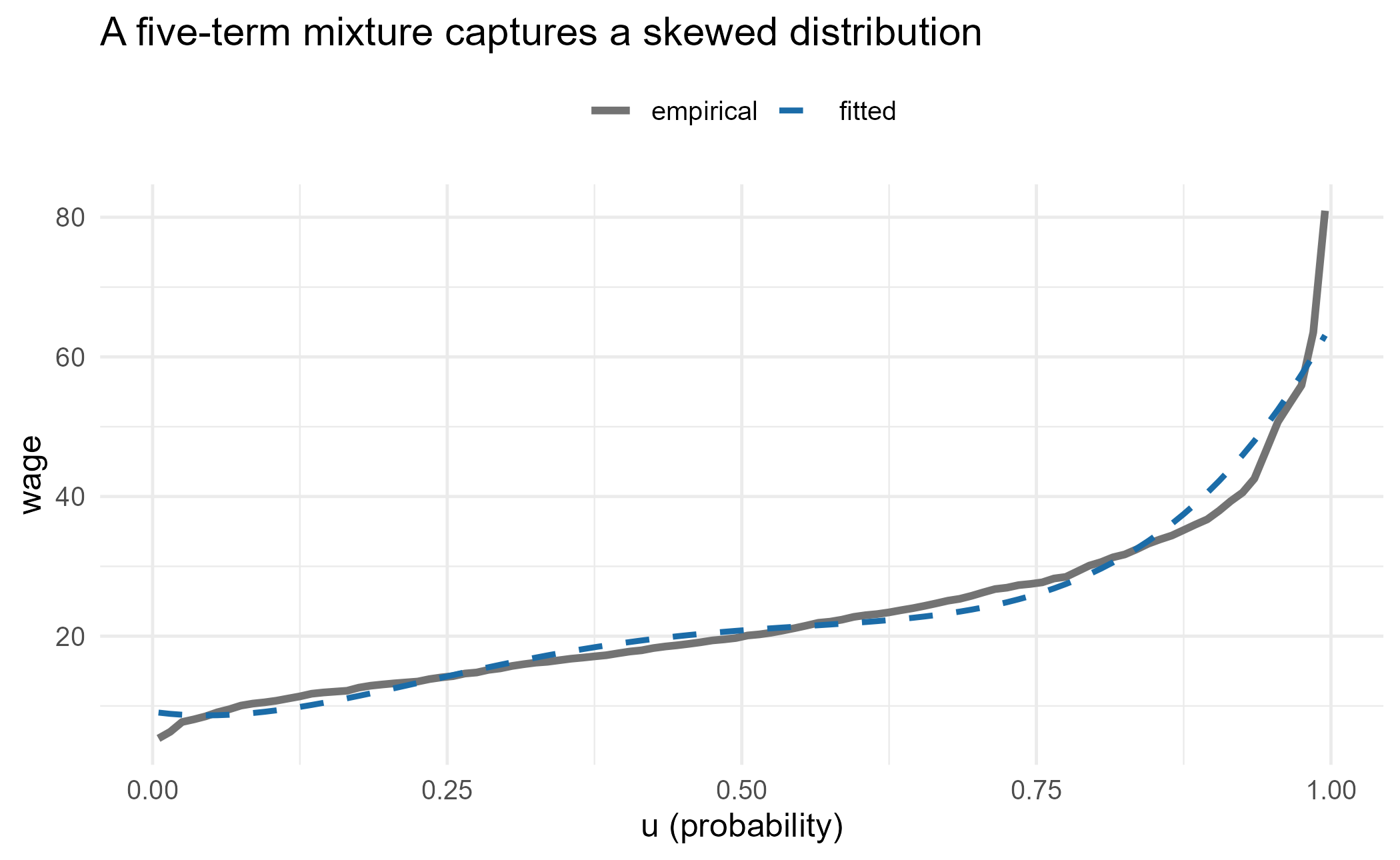
summary() reports how well each L-moment is matched: the
model’s goodness-of-fit.
summary(fit1)
#> Sieve quantile-function mixture (qfmix) -- summary
#>   basis = legendre   p = 5   L = 7   constraint = unconstrained   edf = 5
#>   GMLM objective = -335.9
#>
#> L-moment match (first few):
#>     sample  fitted residual
#> L1 22.8267 22.8267   0.0000
#> L2 11.0892 11.0892   0.0000
#> L3  3.7174  3.7174   0.0000
#> L4  3.2157  3.2157   0.0000
#> L5  1.9138  1.9138   0.0000
#> L6  1.7398  0.0000   1.7398
#>
#> Weights:
#> [1] 22.8267 11.0892  3.7174  3.2157  1.9138
4. Choosing a basis and a constraint
Two choices.
Basis (the shape vocabulary):
| Basis | Use it when |
|---|---|
legendre |
general-purpose, well-conditioned (the default) |
polynomial |
simple, but ill-conditioned at high p – prefer
legendre
|
pareto, gev
|
heavy tails / tail extrapolation |
empirical |
the building blocks are other units’ distributions (synthetic control) |
Constraint (what the weights may do):
| Constraint | Meaning |
|---|---|
unconstrained |
weights free (signed) |
nonneg |
weights |
ridge |
bounded budget (the synthetic-control default) |
simplex |
weights summing to 1 (classic synthetic-control weights) |
The individual weights of a correlated basis are weakly identified, but the fitted quantile function is stable, so judge a fit by the curve and the L-moment match, not by single coefficients.
5. Uncertainty: the numerical bootstrap
qfmix_boot() simulates the sampling law of the fit and
returns a band for the quantile function. Ask for a
uniform (simultaneous) band when you want a statement
that holds across the whole curve at once (Chernozhukov, Chetverikov, and Kato 2014).
bt <- qfmix_boot(fit1, S = 400, target = "quantile", band = "uniform", u = u)
ggplot(data.frame(u = u, est = bt$estimate, lo = bt$lower, hi = bt$upper),
       aes(u, est)) +
  geom_ribbon(aes(ymin = lo, ymax = hi), fill = blue, alpha = 0.2) +
  geom_line(colour = blue, linewidth = 1.1) +
  labs(x = "u", y = "wage",
       title = "Fitted wage quantiles with a 95% simultaneous band")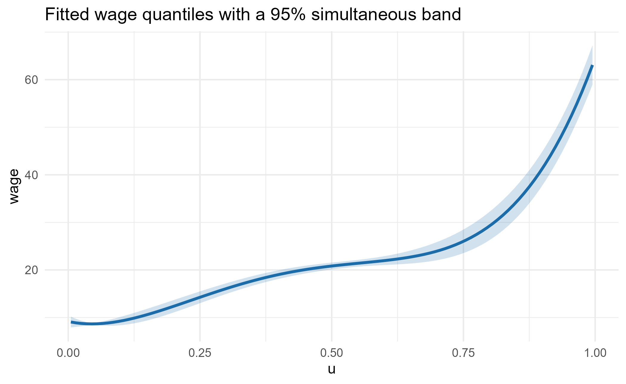
6. The main event: a distributional synthetic control
Now the policy question. One region (the treated unit) adopts a wage floor; we want its effect across the wage distribution. We build a counterfactual from control regions that did not, using their wage distributions as the basis: the empirical-basis case from the table above, and the construction of Gunsilius’s distributional synthetic control (Gunsilius 2023). From here on we work on the log-wage scale.
We first simulate a panel: six control regions and one treated region observed over five years. The treated region’s pre-policy wages are a blend of two control regions (so the controls can reproduce it); from 2019 a floor at the 30th percentile lifts its lower tail.
mk <- function(id, year, v) data.frame(region = id, year = year, logwage = v)
controls <- do.call(rbind, Map(function(j, mu)
  do.call(rbind, lapply(2016:2020, function(t) mk(j, t, rnorm(250, mu, 0.45)))),
  paste0("region", 1:6), c(2.6, 2.8, 3.0, 3.1, 3.3, 3.5)))
treated <- do.call(rbind, lapply(2016:2020, function(t) {
  base <- ifelse(runif(250) < 0.5, rnorm(250, 2.8, 0.45), rnorm(250, 3.1, 0.45))
  if (t >= 2019) base <- pmax(base, quantile(base, 0.30))   # wage floor at p30
  mk("treated", t, base)
}))
panel <- rbind(controls, treated)
One call fits the weights on the pre-policy year
(t0 = 2018) and builds post-policy counterfactuals with
confidence bands.
fit_dsc <- dsc(panel, "region", "year", "logwage",
               treated = "treated", t0 = 2018,
               constraint = "ridge", M = 1, S = 300,
               band = "uniform", bias_aware = TRUE)
fit_dsc
#> Distributional synthetic control (qfmix_dsc)
#>   treated = treated   t0 = 2018   #controls = 6   constraint = ridge
#>   pre-treatment quantile RMSE = 0.02378
#>   bands: uniform, bias-aware
#>   post periods: 2019, 2020
The pre-treatment quantile RMSE is the central credibility check: it says how well the control mixture reproduced the treated distribution before any policy. A small value means the controls span the treated unit.
7. Reading and visualising the effect
summary() reports the distributional treatment effect
(observed minus counterfactual quantile) by percentile and period.
summary(fit_dsc)
#> Distributional treatment effects (observed - counterfactual quantile):
#>
#> period 2019:
#>  percentile effect
#>          10  0.127
#>          25 -0.096
#>          50 -0.163
#>          75 -0.196
#>          90 -0.281
#>
#> period 2020:
#>  percentile effect
#>          10  0.349
#>          25  0.032
#>          50 -0.050
#>          75 -0.094
#>          90 -0.128
A wage floor should show its largest effect at the bottom of the distribution, shrinking toward the top as the floor stops binding. The plot makes it concrete: observed versus counterfactual quantile, then the effect with its band.
pr <- fit_dsc$periods[["2019"]]
ggplot(data.frame(u = pr$u, observed = pr$Qobs, counterfactual = pr$Qcf), aes(u)) +
  geom_line(aes(y = observed, colour = "observed"), linewidth = 1.2) +
  geom_line(aes(y = counterfactual, colour = "counterfactual"), linewidth = 1.2) +
  scale_colour_manual(values = c(observed = "black", counterfactual = blue), name = NULL) +
  labs(x = "u", y = "log wage", title = "Observed vs counterfactual wages (2019)") +
  theme(legend.position = "top")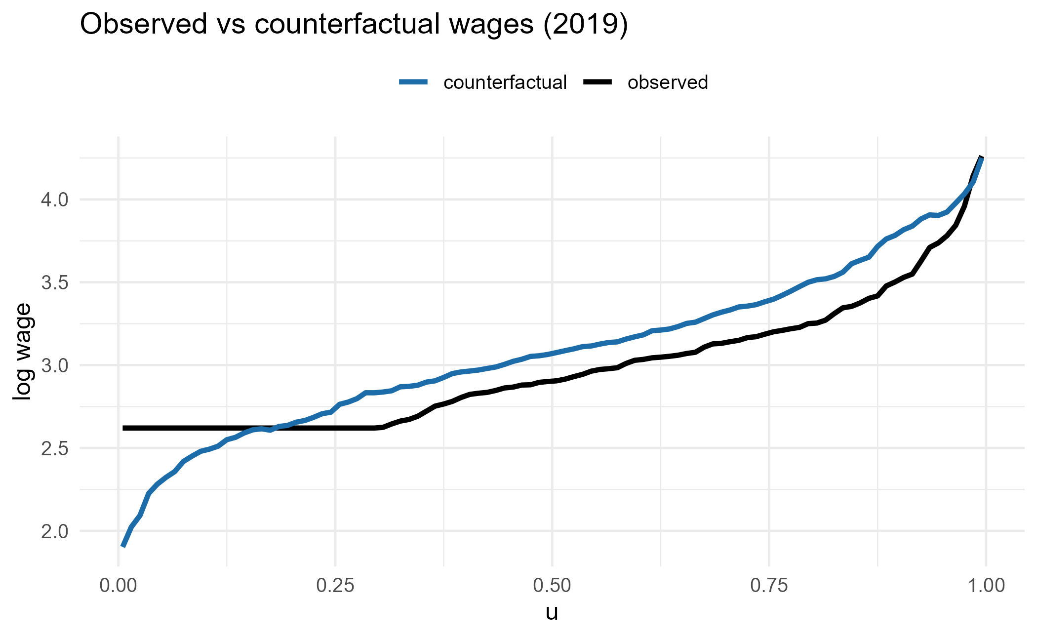
ggplot(data.frame(u = pr$u, eff = pr$effect,
                  lo = pr$band$eff_lower, hi = pr$band$eff_upper), aes(u, eff)) +
  geom_ribbon(aes(ymin = lo, ymax = hi), fill = orange, alpha = 0.2) +
  geom_line(colour = orange, linewidth = 1.2) +
  geom_hline(yintercept = 0, linetype = 3) +
  labs(x = "u (probability)", y = "observed - counterfactual log wage",
       title = "The wage floor lifts the bottom of the distribution",
       subtitle = "Distributional treatment effect, 2019, with 95% band")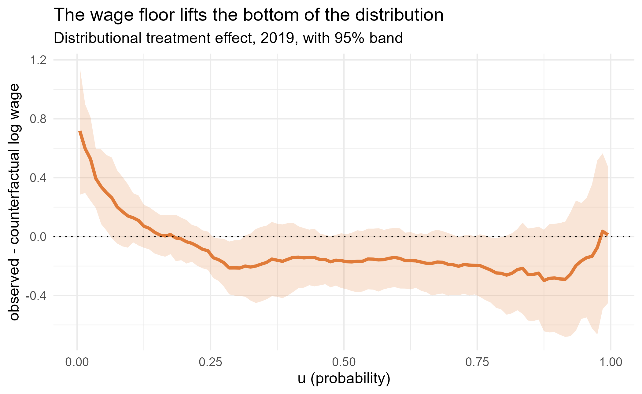
Where the band sits above zero, the policy raised wages; where it straddles zero, there is no detectable effect. The wage floor shows a clear, statistically distinguishable lift at the bottom of the distribution. Higher up, where the floor no longer binds, the effect is small and the band overlaps zero. (The post-period quantiles are re-estimated each run, so the exact numbers shift slightly from seed to seed; read the shape, not a single figure.)
8. Getting coverage right
Two options make the bands trustworthy, and both are on by default in the call above.
-
bias_aware = TRUEwidens the bands by the pre-treatment approximation error. Where the control mixture cannot quite reproduce the treated distribution (typically the tails), variance-only bands are too narrow; this is a conservative bias bound in the spirit of honest-CI inference (Armstrong and Kolesár 2018). It is aqfmixextension: the source paper notes but does not pursue bias-aware inference. -
band = "uniform"gives a simultaneous band valid across the whole quantile curve at once, rather than at each point separately (Chernozhukov, Chetverikov, and Kato 2014).
In Monte-Carlo checks reported in the package NEWS, the
two together lift counterfactual coverage from 0.69 (variance-only,
pointwise) to roughly the nominal 0.95. Two refinements remain open and
are documented in ?dsc: the control-sampling variance and
the exact ridge-ball anti-concentration constant. The
sqrt(n) scaling assumes a donor-pool dilution condition
(Ferman 2021).
9. Diagnostics: can you trust it?
Section 8 made the bands trustworthy; this section checks the fit underneath them.
-
Pre-treatment fit.
fit_dsc$pretreat_rmse(on the log-wage scale) should be small; a large value means the controls do not span the treated distribution and the counterfactual is an extrapolation. Check it before anything else. -
L-moment match. For a plain
qfmixfit,summary()shows the residual between sample and fitted L-moments: the goodness-of-fit. -
Conditioning. Prefer
legendreoverpolynomial; the package warns when a monomial basis is ill-conditioned. -
Monotonicity. A valid quantile function is
nondecreasing;
monotone = TRUEenforces it on a grid for signed-weight fits.
10. Practical guidance and pitfalls
- Judge fits by the curve and the L-moment match (Section 4), not single weights: correlated bases leave individual unstable while the quantile function is well determined.
- For synthetic controls, the pre-treatment RMSE (Section 9) comes first. If the controls cannot reproduce the treated distribution before the policy, no method can trust the counterfactual after it.
- Report bias-aware, uniform bands (Section 8) for any inferential claim; the pointwise variance-only band under-covers in the tails.
-
Use
ridge(the default) orsimplexfor synthetic controls; signed weights extrapolate aggressively and can leave the valid-quantile region. -
Tail questions need tail-aware bases
(
gev,pareto) and sensibletrimming.
11. How qfmix relates to other tools
-
DiSCosimplements Gunsilius’s distributional synthetic control with placebo/permutation inference;qfmixadds the L-moment sieve estimator, signed/ridge weights, and strong-approximation confidence bands (Gunsilius 2023). -
Synth/gsynthare mean-only synthetic controls (Abadie, Diamond, and Hainmueller 2010);qfmixtargets the whole distribution. -
Lmomentsfits a fixed quantile mixture by L-moments (Karvanen 2006);qfmixadds a growing (sieve) basis, convex constraints, and inference. - For single-distribution quantile regression with
covariates, see
quantreg(Koenker 2005) and the companionmixqr/mixqrgatepackages (finite mixtures of quantile regressions).
12. Reporting and reproducibility
qs <- c(0.1, 0.5, 0.9)
eff_q <- pr$effect[vapply(qs, function(q) which.min(abs(pr$u - q)), integer(1))]
list(weights = round(fit_dsc$weights, 3),
     pretreat_rmse = round(fit_dsc$pretreat_rmse, 3),
     effect_at_10_50_90 = round(setNames(eff_q, paste0("p", qs * 100)), 3),
     bands = paste0(fit_dsc$band, if (fit_dsc$bias_aware) ", bias-aware"))
#> $weights
#> [1]  0.407 -0.108  0.837 -0.022  0.242 -0.283
#>
#> $pretreat_rmse
#> [1] 0.024
#>
#> $effect_at_10_50_90
#>    p10    p50    p90
#>  0.127 -0.163 -0.281
#>
#> $bands
#> [1] "uniform, bias-aware"
Report: the control weights and the constraint used; the pre-treatment fit quality; the distributional effect by percentile with bands; and the band type (uniform, bias-aware) so readers know what the intervals cover.