Location-varying gating for mixtures of quantile regressions

Kailas Venkitasubramanian, University of North Carolina at Charlotte

A finite mixture of quantile regressions splits the data into latent groups and fits a quantile regression in each (see the mixqr package). The mixing probabilities are usually a single set of constants. mixqrgate lets them depend on covariates through a multinomial-logit gate, and lets the gate change with the quantile level – so membership itself can shift across the conditional distribution (Furno 2025).

The contribution over Furno’s reweighting heuristic is inference: the gate is the maximiser of the mixture Q-function, so it comes with standard errors. You can ask whether membership depends on a covariate, and whether it varies across the distribution, rather than eyeballing a curve.

library(mixqrgate)
library(ggplot2)

A concomitant gate

sim_gate2() simulates two components whose membership depends on a gating covariate z: Pr(class 2 | z) = plogis(0 + 1.5 z). The components are quantile regressions of y on x with slopes -3 and +3.

d <- sim_gate2(n = 600, gamma = c(0, 1.5))
fit <- mixqrgate(y ~ x, data = d, gating = ~ z, G = 2, tau = 0.5,
                 variance = "louis")
summary(fit)
#> Gated mixture of quantile regressions (mixqrgate) -- summary
#>   G = 2   method = ald   gating: ~z
#> 
#> ===== tau = 0.5 =====
#> Component coefficients:
#>               comp1   comp2
#> (Intercept)  1.9696 -2.1050
#> x           -2.9306  3.1227
#> 
#> Gate coefficients (membership vs gating covariates):
#>                   Estimate Std.Err z value Pr(>|z|)    
#> comp2:(Intercept)  -0.1009  0.1204  -0.838    0.402    
#> comp2:z             1.7178  0.1849   9.291   <2e-16 ***
#> ---
#> Signif. codes:  0 '***' 0.001 '**' 0.01 '*' 0.05 '.' 0.1 ' ' 1
#> logLik = -1216.20   AIC = 2448.4   BIC = 2483.6
#> 
#> Gate SEs: louis (classification-aware).

The component slopes are recovered (about -3 and +3), and the gate coefficient on z (component 2 vs. component 1) is positive and significant: higher z raises the odds of the second regime, as simulated. We used variance = "louis", the Louis observed-information standard error that accounts for uncertainty about which observation belongs to which class (in simulations it reaches nominal coverage where the default sandwich SE, conditional on the fitted memberships, reaches only about 0.80). variance = "stochEM" is a multiple-imputation alternative. Setting gating = ~1 recovers a constant gate and the ordinary mixqr fit.

Does the gate vary with the quantile?

With vary_gating = "discrete" the gate is fit separately at each quantile. The key point is that each gate carries its own uncertainty – so the question “does membership vary across the distribution?” is answered with inference, not by reading a noisy curve.

dh <- sim_gate2(n = 1000, gamma = c(0, 1), sigma = c(1, 3),
                loc_vary = 2.5, het = TRUE)               # location-coupled gate
fitv <- mixqrgate(y ~ x, data = dh, gating = ~ z, G = 2,
                  tau = c(0.1, 0.25, 0.5, 0.75, 0.9),
                  vary_gating = "discrete")
round(fitv$gate_prob, 3)
#>        [,1]  [,2]  [,3]  [,4] [,5]
#> comp1 0.463 0.471 0.503 0.537 0.55
#> comp2 0.537 0.529 0.497 0.463 0.45

We draw the class-average gate probability at each $\tau$ with an uncertainty band (simulated from each gate’s covariance), so the eye is not fooled by sampling noise.

gate_band <- function(fit, comp = 2, R = 400) {
  do.call(rbind, lapply(seq_along(fit$tau_grid), function(g) {
    gam <- as.numeric(fit$gamma[, , g]); V <- fit$gate_vcov[[g]]
    L <- chol(V + 1e-8 * diag(nrow(V)))
    draws <- sapply(seq_len(R), function(r) {
      gd <- matrix(gam + as.numeric(crossprod(L, rnorm(length(gam)))),
                   length(fit$znames))
      mean(mixqrgate:::gate_predict(gd, fit$z)[, comp])
    })
    data.frame(tau = fit$tau_grid[g], prob = mean(draws),
               lo = quantile(draws, .025), hi = quantile(draws, .975))
  }))
}
gb <- gate_band(fitv)

ggplot(gb, aes(tau, prob)) +
  geom_ribbon(aes(ymin = lo, ymax = hi), fill = "#1b6ca8", alpha = 0.2) +
  geom_line(linewidth = 1.1, colour = "#1b6ca8") +
  geom_point(size = 2.4, colour = "#1b6ca8") +
  ylim(0, 1) +
  labs(x = expression(tau), y = "Class-average gate probability (component 2)",
       title = "Is the gate location-varying?",
       subtitle = "Point estimates per quantile, with simulated uncertainty bands") +
  theme_minimal(base_size = 12)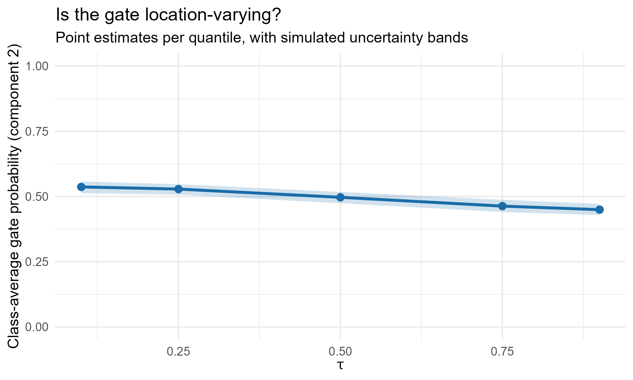

Read with its uncertainty, the gate drifts only modestly here, and the bands at neighbouring quantiles overlap – the evidence for a location-varying gate in this sample is weak. That is the right answer to report: the per-quantile gates are fit independently and are genuinely noisy (the “classification ambiguity across $\tau$” of Wu & Yao 2016), and the method does not manufacture a trend. On data with strong location-varying mixing – Furno’s PISA example, where the best-performing class dominates the lower tail and the worst the upper – the same machinery surfaces it, and the per-$\tau$ gate coefficients with their standard errors (summary(fitv)) let you test it formally. Borrowing strength across neighbouring $\tau$ with a smooth gate (a planned vary_gating = "smooth" mode) will sharpen this where the discrete fit is noisy.

Notes

• method = "kde" uses the Wu & Yao (2016) nonparametric error densities instead of the parametric asymmetric-Laplace path. Gate SEs there are not yet classification-aware; treat them as approximate.
• The gating covariates may be the same as, overlap with, or be disjoint from the component-regression covariates.
• predict(fit, newdata, type = "prob", tau = 0.9) returns the gate probabilities at a chosen quantile for new data; confint(fit) gives gate-coefficient intervals.

References

• Furno, M. (2025). Finite Mixture at Quantiles and Expectiles. Journal of Risk and Financial Management 18(4), 177.
• Wu, Q. & Yao, W. (2016). Mixtures of quantile regressions. Computational Statistics & Data Analysis 93, 162–176.
• Grün, B. & Leisch, F. (2008). FlexMix version 2. Journal of Statistical Software 28(4), 1–35.