A Primer on Location-Varying Gating for Quantile Mixtures

This primer is for applied researchers (in education, economics, sociology, public health) who suspect their population is a mixture of latent groups, who care about the whole distribution of an outcome rather than its average, and who want to know whether group membership itself changes across that distribution. No background in mixture models or quantile regression is assumed. By the end you will be able to fit the model, read every number it returns, judge whether to trust it, and report it responsibly.

library(mixqrgate)
library(ggplot2)

pal <- c("Supportive" = "#1b6ca8", "Under-resourced" = "#e07b39")
theme_set(theme_minimal(base_size = 12))

1. The question

Imagine test scores from many schools. Two stories could be true at once:

One population, unequal returns. Family socio-economic status (SES) raises scores, more steeply at the bottom of the distribution than at the top.
Two kinds of school. Some schools are under-resourced: scores track SES steeply, so advantaged children pull far ahead. Others are supportive: the SES gradient is flatter and the baseline higher, so the school compensates.

If the second story holds, two further questions follow. Which schools are which, and what predicts it? And – the question this package is built for – does the mix change across the score distribution? A school might look supportive among its low scorers and under-resourced among its high scorers. That is location-varying mixing (Furno 2025), and until now it had no inferential tool in R.

2. The model in one page

We model the conditional quantile of the outcome, not its mean. The -th quantile ( is the median) of score given SES is a mixture of latent regimes (Wu and Yao 2016):

In regime , the -th quantile is linear in SES, , estimated by minimising the check loss (Koenker and Bassett 1978), the workhorse of quantile regression (Koenker 2005).
A school belongs to regime with probability . In an ordinary mixture these mixing weights are constants. Here they follow a multinomial-logit gate on gating covariates (e.g. school funding): This is the concomitant-variable idea of Grün and Leisch (2008), here attached to quantile components.
The new move: the gate coefficients may carry a argument, , so the mix can shift across the distribution.

Estimation is by EM (McLachlan and Peel 2000). The gate step is a weighted multinomial logistic regression of the soft group labels on , the principled replacement for Furno’s reweighting heuristic, and what lets us put standard errors on the gate (Section 6 discusses making those errors trustworthy). Setting gating = ~1 removes the gate and recovers an ordinary mixture of quantile regressions.

3. An illustrative dataset

sim_gate2() generates this structure. We rename its columns to the schools story: score, ses, and funding (the gating covariate). Two regimes differ in their SES gradient; funding raises the odds of the supportive regime.

raw <- sim_gate2(n = 800, gamma = c(-0.3, 1.3),
                 b1 = c(48, 7), b2 = c(55, 2), sigma = c(6, 7))
schools <- data.frame(score = raw$y, ses = raw$x, funding = raw$z)
head(round(schools, 2))
#>   score   ses funding
#> 1 56.75  0.62   -0.14
#> 2 41.60  0.04   -0.26
#> 3 57.23  0.77    1.21
#> 4 61.48  1.27    0.07
#> 5 57.90  0.37    0.44
#> 6 57.04 -0.16    0.31

The two regimes overlap heavily in the raw scatter, which is the whole problem. You cannot eyeball the groups; you need a model to recover them.

# class 1 is, by construction, the steep-gradient (under-resourced) regime
schools$truth <- ifelse(raw$class == 1, "Under-resourced", "Supportive")
ggplot(schools, aes(ses, score, colour = truth)) +
  geom_point(alpha = 0.5, size = 1.3) +
  scale_colour_manual(values = pal, name = "True regime") +
  labs(x = "Student SES (standardised)", y = "Test score",
       title = "Two regimes are present but entangled") +
  theme(legend.position = "top")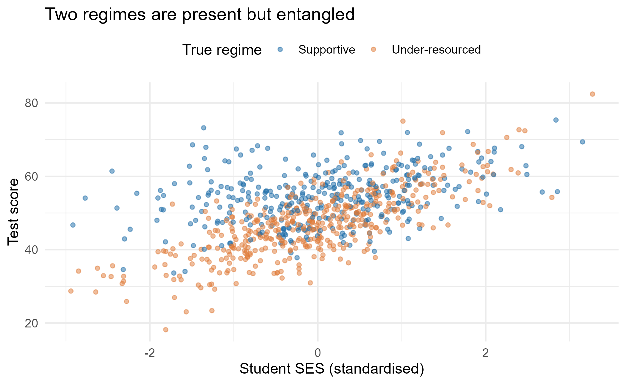

Scatter of score against SES, two latent regimes overlapping.

4. Fitting your first model

One call. We fit two regimes at the median, gate on funding, and ask for the Louis standard errors (Section 6 explains the choice).

fit <- mixqrgate(score ~ ses, data = schools, gating = ~ funding,
                 G = 2, tau = 0.5, variance = "louis")
fit
#> Gated mixture of quantile regressions (mixqrgate)
#>   components G = 2   method = ald   n = 800
#>   tau grid: 0.5   gating: ~funding
#>   vary_gating = none
#> 
#> Class-average gate probabilities (rows = components, cols = tau):
#>       tau=0.5
#> comp1  0.3104
#> comp2  0.6896
#> 
#> Component coefficients at tau = 0.5 :
#>               comp1   comp2
#> (Intercept) 56.3228 47.7420
#> ses          2.3795  6.3602

print shows the class-average gate probabilities and the component coefficients. Components are ordered by their SES slope, so component 1 is always the flatter-gradient supportive regime and component 2 the steeper under-resourced one. The estimated slopes recover the two true gradients: the flatter near 2, the steeper near 6–7.

5. Interpreting the gate

summary() adds the piece Furno’s method cannot: the gate coefficients with standard errors.

summary(fit)
#> Gated mixture of quantile regressions (mixqrgate) -- summary
#>   G = 2   method = ald   gating: ~funding
#> 
#> ===== tau = 0.5 =====
#> Component coefficients:
#>               comp1   comp2
#> (Intercept) 56.3228 47.7420
#> ses          2.3795  6.3602
#> 
#> Gate coefficients (membership vs gating covariates):
#>                   Estimate Std.Err z value Pr(>|z|)    
#> comp2:(Intercept)   0.9945  0.1619   6.143 8.11e-10 ***
#> comp2:funding      -1.1706  0.1956  -5.984 2.18e-09 ***
#> ---
#> Signif. codes:  0 '***' 0.001 '**' 0.01 '*' 0.05 '.' 0.1 ' ' 1
#> logLik = -2698.59   AIC = 5413.2   BIC = 5450.7
#> 
#> Gate SEs: louis (classification-aware).

Read the gate block as a logistic regression for being in component 2 (under-resourced) rather than component 1 (supportive). The coefficient on funding is negative and significant: better-funded schools are less likely to be in the steep-gradient regime. Exponentiate it for an odds ratio.

g <- coef(fit, "gating")["funding", 1, 1]
cat(sprintf("odds ratio per 1 SD of funding: %.2f\n", exp(g)))
#> odds ratio per 1 SD of funding: 0.31
confint(fit)        # gate-coefficient confidence intervals
#>                         2.5%      97.5%
#> comp2:(Intercept)  0.6771758  1.3117949
#> comp2:funding     -1.5539867 -0.7871582

The class-average gate probabilities (fit$gate_prob) summarise the mix; the per-school probabilities live in predict(fit, type = "prob").

But before we trust that coefficient, the standard error behind it has to be sound, which in a mixture is less obvious than it looks.

6. Getting the uncertainty right

A mixture never knows for certain which group an observation belongs to. A naive standard error that ignores this – the default "sandwich", computed as if memberships were known – is too small and under-covers. mixqrgate offers two classification-aware alternatives:

variance = "louis" – an analytic observed-information correction (Louis 1982) that subtracts the “missing information” from the latent labels. Fast, and the recommended default for inference.
variance = "stochEM" – a multiple-imputation estimate (Little and Rubin 2002): draw labels, refit the gate, combine. Slower, a useful cross-check.

The difference is not cosmetic. The conditional sandwich under-covers (in a Monte-Carlo check it held a nominal 95% interval only about 80% of the time), and the Louis correction is designed to give back exactly the coverage the sandwich loses (in the same check it returned the interval to roughly nominal).

se <- function(v) sqrt(diag(vcov(mixqrgate(score ~ ses, data = schools,
        gating = ~ funding, G = 2, tau = 0.5, variance = v,
        control = mixqrgate_control(seed = 1)))))
rbind(sandwich = se("sandwich"), louis = se("louis"))
#>                [,1]       [,2]
#> sandwich 0.05081167 0.05661757
#> louis    0.16189560 0.19562312

The Louis standard errors are larger: the real cost of not knowing the labels.

7. Does membership shift across the distribution?

Now the headline question. We need data in which the answer is yes: where a school’s regime depends on where its students sit in the score distribution. sim_gate2(loc_vary = 3) builds that: membership is tied to the quantile rank, so the under-resourced regime is scarce among low scorers and common higher up. (With loc_vary = 0, the package default, the mix is constant across ; the tool should – and does – report no shift there.)

lv <- sim_gate2(n = 800, gamma = c(-0.3, 1.3),
                b1 = c(48, 7), b2 = c(55, 2), sigma = c(6, 7), loc_vary = 3)
schools_lv <- data.frame(score = lv$y, ses = lv$x, funding = lv$z)

Pass a grid of quantiles with vary_gating = "discrete"; the gate is refit at each. Each gate carries its own uncertainty, so “does the mix change with the quantile?” is answered with inference, not by eyeballing a wiggly line.

grid <- c(0.1, 0.25, 0.5, 0.75, 0.9)
fitv <- mixqrgate(score ~ ses, data = schools_lv, gating = ~ funding,
                  G = 2, tau = grid, vary_gating = "discrete",
                  variance = "louis")
round(fitv$gate_prob, 3)
#>        [,1] [,2]  [,3]  [,4]  [,5]
#> comp1 0.692 0.29 0.398 0.488 0.422
#> comp2 0.308 0.71 0.602 0.512 0.578

We need uncertainty on each point. At every we draw many plausible gates from that fit’s covariance and record the spread of the implied class share, so the ribbon shows sampling noise, not just the point estimate.

band <- do.call(rbind, lapply(seq_along(grid), function(g) {
  V <- fitv$gate_vcov[[g]]; gam <- as.numeric(fitv$gamma[, , g])
  L <- chol(V + 1e-8 * diag(nrow(V)))
  d <- replicate(500, {
    gd <- matrix(gam + as.numeric(crossprod(L, rnorm(length(gam)))),
                 length(fitv$znames))
    mean(mixqrgate:::gate_predict(gd, fitv$z)[, 2])
  })
  data.frame(tau = grid[g], p = mean(d),
             lo = quantile(d, .025), hi = quantile(d, .975))
}))

ggplot(band, aes(tau, p)) +
  geom_ribbon(aes(ymin = lo, ymax = hi), fill = pal[2], alpha = 0.2) +
  geom_line(colour = pal[2], linewidth = 1.1) +
  geom_point(colour = pal[2], size = 2.3) +
  ylim(0, 1) +
  labs(x = expression(tau), y = "P(under-resourced regime)",
       title = "The mix shifts across the score distribution",
       subtitle = "Per-quantile gate estimates, with simulated uncertainty")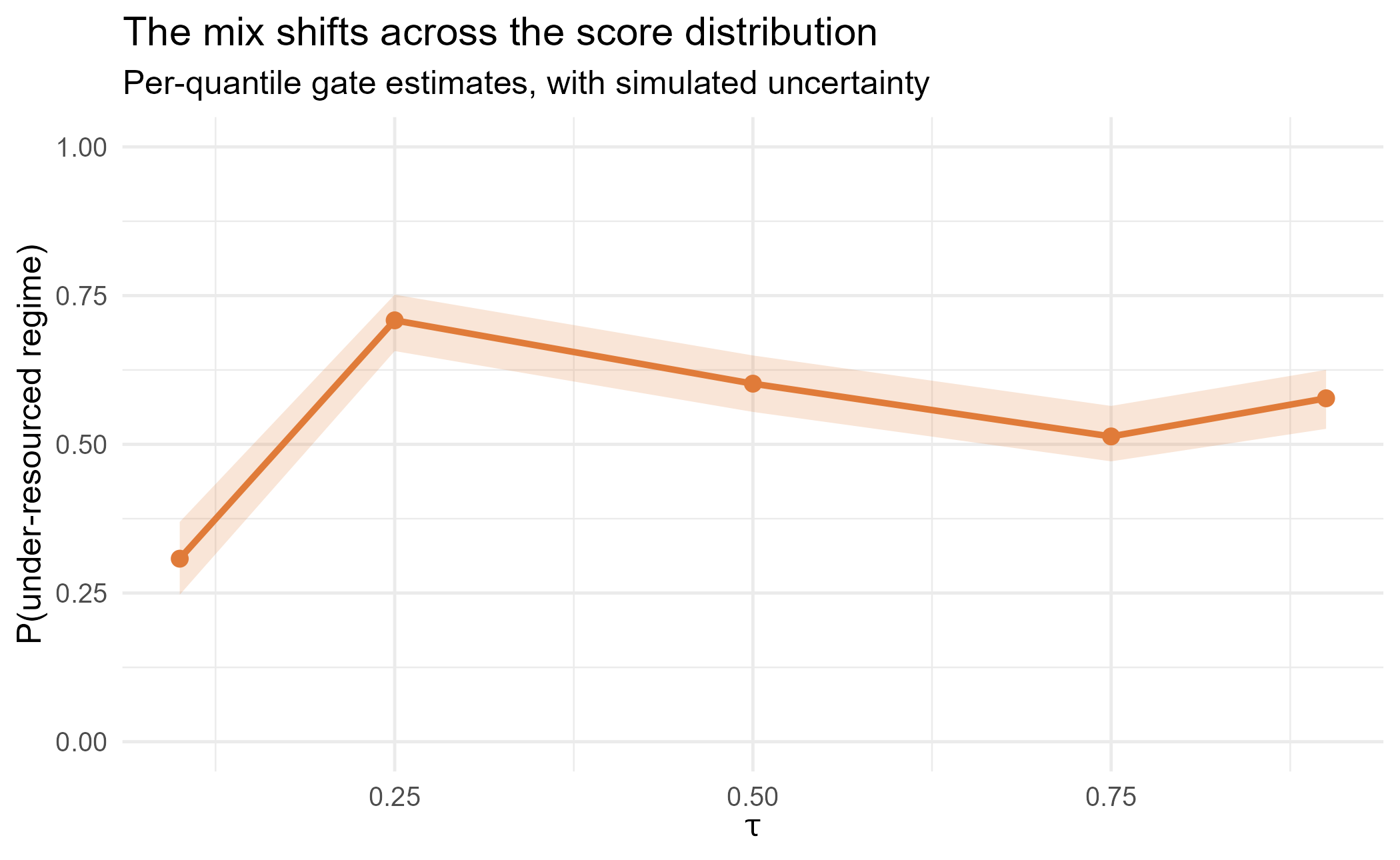

Average gate probability against the quantile level with uncertainty bands.

The under-resourced regime is least common in the lower tail and more common through the middle and upper range: the location-varying mixing built into the data, recovered by the model. Two cautions keep the reading sober. First, the per-quantile gates are fit independently and are noisy (the “classification ambiguity across ” of Wu and Yao (2016)), so neighbouring points wobble; lean on the bands, not the dots. Second, on data with a constant true gate (loc_vary = 0) this same picture comes out flat within its uncertainty; the method does not manufacture a trend. The value of the tool is that it lets you test the question with standard errors rather than over-reading a curve; summary(fitv) reports the gate coefficients with their SEs at each for that.

8. Reading the fit in pictures

Two pictures earn their place here. (The regimes themselves are just the two fitted median gradients – slopes near 2 and 6–7, already printed in Section 4 – so we do not re-draw the scatter.)

Who is in which group? Posterior probabilities express the (ir)reducible uncertainty of assignment.

schools$p_under <- fit$posterior[, 2, 1]
ggplot(schools, aes(ses, score, colour = p_under)) +
  geom_point(size = 1.4) +
  scale_colour_gradient(low = pal[1], high = pal[2],
                        name = "P(under-resourced)") +
  labs(x = "Student SES", y = "Test score",
       title = "Soft classification: confident at the edges, unsure in the middle")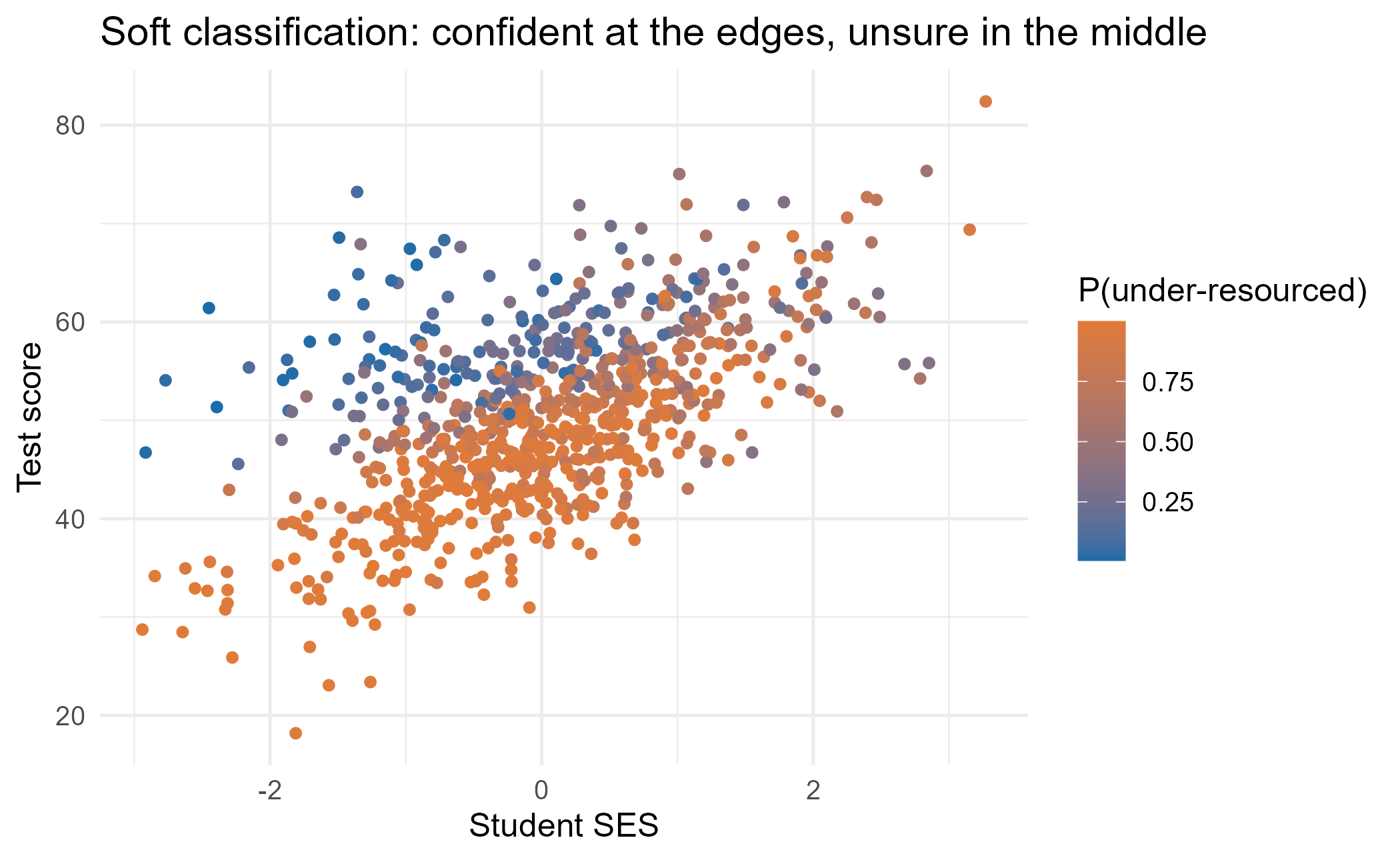

Posterior probability of the under-resourced regime across the data.

The gate as a curve. Because the gate is a logistic model on funding, we can draw the fitted regime probability against funding directly.

nd <- data.frame(funding = seq(-2.5, 2.5, length.out = 100))
pp <- predict(fit, newdata = nd, type = "prob")
gd <- data.frame(funding = rep(nd$funding, 2),
                 prob = c(pp[, 1], pp[, 2]),
                 regime = rep(c("Supportive", "Under-resourced"), each = 100))
ggplot(gd, aes(funding, prob, colour = regime)) +
  geom_line(linewidth = 1.2) +
  scale_colour_manual(values = pal, name = NULL) +
  labs(x = "School funding (standardised)", y = "Gate probability",
       title = "The gate: funding shifts the regime mix") +
  theme(legend.position = "top")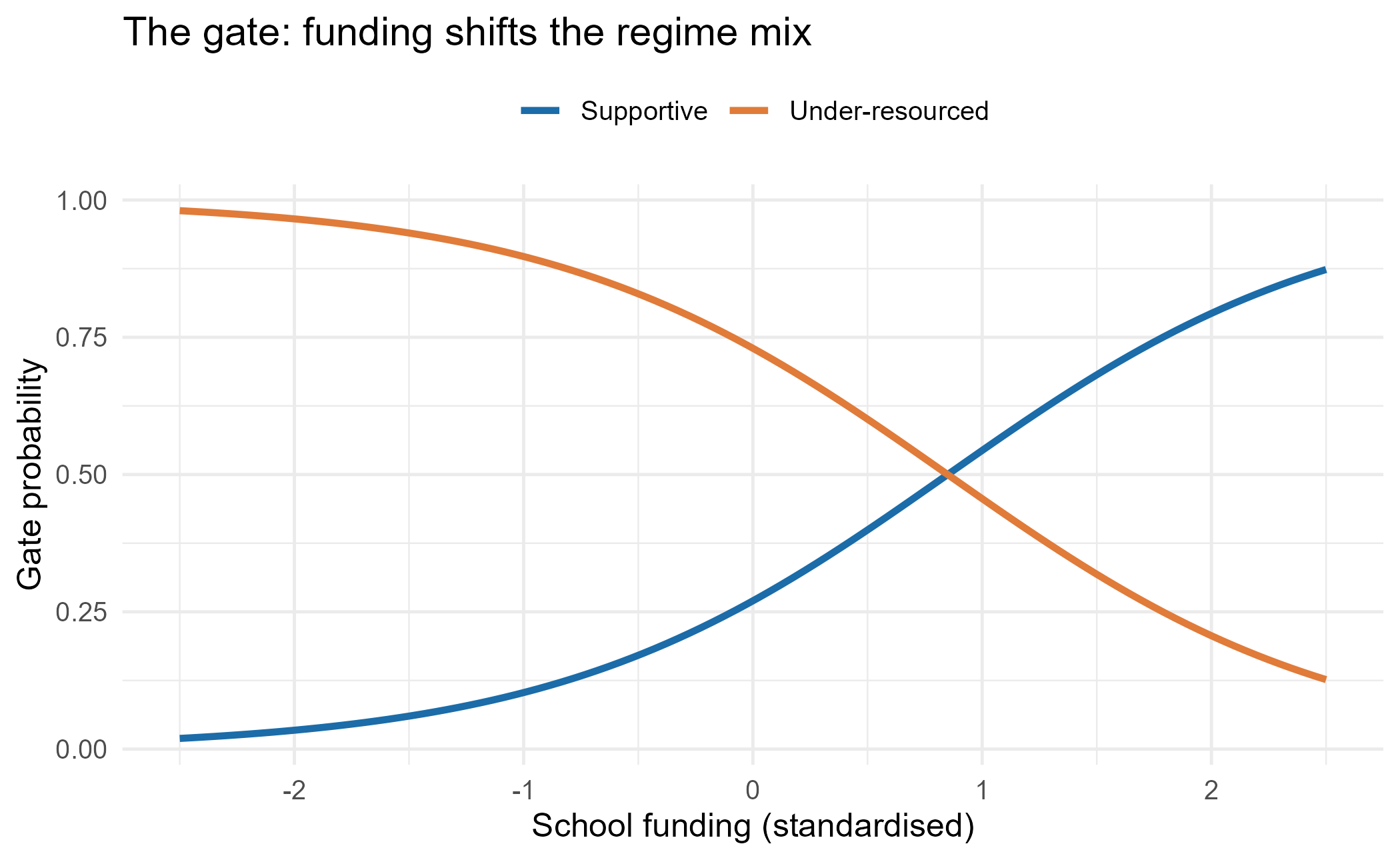

Fitted probability of each regime as a function of school funding.

9. Diagnostics: can you trust it?

A few checks before believing any mixture fit.

Convergence. fit$converged should be TRUE at every . mixqrgate warns otherwise.
No collapsed component. If a regime’s average gate probability is tiny, the mixture has effectively one component; the package warns. Inspect fit$gate_prob.
A well-conditioned gate. Highly collinear gating covariates make the gate coefficients unstable; fit$gate_cond reports the conditioning and the package warns when it is large.
Distinct components. The regimes must differ (Theorem 2.1 of Wu and Yao (2016)); near-identical slopes are weakly identified.

c(converged = all(fit$converged),
  min_gate_prob = round(min(fit$gate_prob), 3),
  gate_condition = round(fit$gate_cond, 1))
#>      converged  min_gate_prob gate_condition 
#>           1.00           0.31           2.20

Multi-start (the nstart control) guards against local optima; the mixture likelihood is multimodal, so several starts are essential.

10. Practical guidance and pitfalls

Start at the median, gate on a few substantively chosen covariates. A gate with many collinear predictors is hard to identify.
Report Louis (or stochEM) standard errors, never the conditional sandwich, whenever you make an inferential claim about the gate.
Treat the discrete -gate as exploratory. Per-quantile gates are noisy; look at the uncertainty bands and resist over-reading a trend.
Choose for interpretability, not fit alone. Two or three substantively meaningful regimes usually beat a larger number chosen by an information criterion.
The component labels are slope-ordered, so they are stable across runs; describe them by what their slopes mean.

11. How mixqrgate relates to other tools

flexmix has the concomitant multinomial gate but no quantile / check-loss components, so it cannot produce -quantile regimes (Grün and Leisch 2008).
brms can gate on covariates and fix a quantile per component, but cannot make the gate a function of or fit several jointly.
Furno’s (2025) Stata routine is the only prior location-varying-gating tool; it is a reweighting heuristic with no standard errors on the gate. mixqrgate turns that idea into a likelihood/EM object with inference (Furno 2025).
mixqr is the parent: an ordinary mixture of quantile regressions. mixqrgate with gating = ~1 reproduces it (to EM tolerance).

12. Reporting and reproducibility

A compact, reproducible report of the headline fit:

set.seed(2025)
fit_final <- mixqrgate(score ~ ses, data = schools, gating = ~ funding,
                       G = 2, tau = 0.5, variance = "louis",
                       control = mixqrgate_control(seed = 2025))
list(slopes = round(fit_final$beta["ses", , 1], 2),
     gate_funding = round(coef(fit_final, "gating")["funding", 1, 1], 3),
     gate_prob = round(fit_final$gate_prob[, 1], 3),
     se_method = fit_final$se_method)
#> $slopes
#> comp1 comp2 
#>  2.38  6.36 
#> 
#> $gate_funding
#> [1] -1.171
#> 
#> $gate_prob
#> comp1 comp2 
#>  0.31  0.69 
#> 
#> $se_method
#> [1] "louis"

Report: the number of regimes and why; the component gradients; the gate coefficients with their (classification-aware) standard errors and the odds-ratio interpretation; the standard-error method; and, if you used the -grid, the gate-vs- picture with its uncertainty.

That last clause is the whole point. The schools were never labelled; the model recovered two gradients, told us funding predicts which a school follows, and – when the data warranted it – showed the mix shifting across the score distribution. Each of those is a claim with a standard error behind it. The discipline the primer asks for is to read those pictures with their uncertainty, and to test rather than eyeball.

References

Furno, Marilena. 2025. “Finite Mixture at Quantiles and Expectiles.” Journal of Risk and Financial Management 18 (4): 177.

Grün, Bettina, and Friedrich Leisch. 2008. “FlexMix Version 2: Finite Mixtures with Concomitant Variables and Varying and Constant Parameters.” Journal of Statistical Software 28 (4): 1–35.

Koenker, Roger. 2005. Quantile Regression. Cambridge University Press.

Koenker, Roger, and Gilbert Bassett. 1978. “Regression Quantiles.” Econometrica 46 (1): 33–50.

Little, Roderick J. A., and Donald B. Rubin. 2002. Statistical Analysis with Missing Data. 2nd ed. Wiley.

Louis, Thomas A. 1982. “Finding the Observed Information Matrix When Using the EM Algorithm.” Journal of the Royal Statistical Society, Series B 44 (2): 226–33.

McLachlan, Geoffrey J., and David Peel. 2000. Finite Mixture Models. New York: Wiley.

Wu, Qiang, and Weixin Yao. 2016. “Mixtures of Quantile Regressions.” Computational Statistics & Data Analysis 93: 162–76.

Kailas Venkitasubramanian, University of North Carolina at Charlotte