Getting Started with rsdv: A Practitioner's Guide to Synthetic Data Generation

Introduction

Administrative records, survey microdata, and clinical data share a common problem: the very features that make them analytically valuable — individual-level detail, rare subgroup representation, longitudinal linkage — also make them difficult to share. Data governance procedures, informed consent agreements, and privacy regulations all impose friction between the data and the analyst. Synthetic data generation addresses this by learning the statistical structure of a real dataset and using it to generate a new one whose rows are artificial but whose distributional properties approximate the original.

rsdv is an R implementation of the Synthetic Data Vault (SDV) framework (Patki, Wedge, and Veeramachaneni 2016), bringing a Gaussian copula–based synthesis workflow to native R. The package is designed for the applied researcher who needs to generate a shareable analogue of a sensitive dataset, evaluate how closely the synthetic version preserves the real data’s distributions and correlation structure, and quantify the privacy protection the synthesis affords. The workflow follows four steps: describe the column types, fit the synthesizer, generate synthetic rows, and evaluate the result.

---

The R Synthetic Data Ecosystem

Several R packages generate synthetic data, each rooted in a different methodological tradition.

Sequential imputation methods. synthpop (Nowok, Raab, and Dibben 2016) is the most widely cited R synthesis package. It generates synthetic variables one at a time, conditioning each column on those already synthesised using parametric models or classification and regression trees (CART). The sequential approach is flexible and interpretable, and synthpop has mature support for multiple-imputation inference and disclosure risk measurement. It is widely adopted in official statistics, including within UK government data infrastructure. Sequential CART approximates the joint distribution column-by-column rather than modelling it as a single object — so for high-dimensional mixed data, correlation error accumulates across steps.

Adversarial methods. arf (Watson, Blesch, Kapar, and Wright 2023) implements Adversarial Random Forests, which partition the feature space into locally independent leaves by iterating between a forest-based density estimator and a discriminator. On tabular benchmarks it matches or outperforms deep generative models while running roughly 100 times faster — which matters for practitioners without GPU access. It handles mixed variable types naturally. The package is primarily oriented toward ML researchers rather than practitioners in regulated industries; it does not provide metadata schemas, quality reports, or privacy metrics.

Rank-based methods. synthesizer (Van der Loo, Statistics Netherlands) synthesises data using empirical rank-based correlation, with a single rankcor parameter governing the privacy-utility tradeoff. The approach is fast, handles missing data patterns, and is appropriate for settings where a lightweight baseline synthesis is needed. Quality metrics beyond pMSE are not built in.

Disclosure control suites. sdcMicro (Templ, Kowarik, and Meindl 2015) is a comprehensive toolkit for statistical disclosure control, covering suppression, perturbation, microaggregation, and synthesis within a unified framework used by national statistical offices globally. Synthesis in sdcMicro is one method among many; synthesis is not the primary product, and the workflow is designed around disclosure risk assessment and perturbation pipelines rather than generative modeling.

Copula infrastructure. The copula package (Hofert, Kojadinovic, Mächler, and Yan) is the foundational R library for copula families including Gaussian, t, Clayton, Gumbel, Frank, and Joe. rsdv uses copula internally for fitting and sampling. heterocop (Tomilina, Mazo, and Jaffrézic 2024) and GenOrd are methodologically adjacent — both estimate Gaussian copulas for mixed discrete and continuous variables. heterocop targets network inference; GenOrd targets simulation.

Where rsdv fits

rsdv occupies the intersection of properties no single existing package combines: a parametric copula model for joint distribution preservation, first-class support for mixed variable types (continuous, categorical, boolean), an integrated quality and privacy evaluation report, and a tidy metadata → fit → sample → evaluate API. The disclosure control suites (sdcMicro, synthpop) provide privacy metrics within their own frameworks but are not designed around generative modelling as the primary product. rsdv’s architecture is designed so that the Gaussian copula can be replaced by a vine copula or a deep generative model without changing the user-facing interface, providing a clear upgrade path as needs grow.

---

The Gaussian Copula: A Practitioner’s Introduction

A copula is a joint distribution that separates the behaviour of each individual variable from the way variables depend on one another. Sklar’s theorem (Sklar 1959) guarantees that any multivariate distribution can be written as a copula applied to its marginal CDFs. For synthesis, this decomposition is useful: we can estimate the dependence structure from data and then recombine it with estimated or empirical marginal distributions to generate new observations.

The Gaussian copula models dependence through a correlation matrix. The synthesis pipeline has five stages:

1. Transform to uniform. Each numerical value is mapped to the interval (0, 1) through its fitted marginal CDF (the probability integral transform). rsdv fits a parametric family per column — norm, beta, gamma, truncnorm, or uniform — and by default (default_distribution = "auto") selects the best-fitting family by Kolmogorov-Smirnov distance. You can override the choice per column via numerical_distributions. Categorical and boolean columns are mapped to (0, 1) by their cumulative-frequency intervals (each value is placed uniformly at random within its category’s interval), so they enter the copula too.

2. Map to normal space. The uniform values are passed through the standard normal quantile function (Φ⁻¹), yielding pseudo-observations on the real line.

3. Estimate the correlation matrix. The correlation matrix of the normal-space pseudo-observations is estimated using inversion of Kendall’s τ, a rank-based method that is more stable than maximum likelihood for small samples or tied values.

4. Sample. New pseudo-observations are drawn from the fitted multivariate normal distribution.

5. Back-transform. Numerical columns are mapped back through their fitted quantile function; categorical and boolean columns are decoded by locating which frequency interval each sampled value falls into.

Because the copula embeds every column — numerical, categorical, and boolean — it preserves cross-type dependence: numeric-vs-categorical and categorical-vs-categorical associations, not just numeric-vs-numeric correlations.

rsdv fits the copula on complete cases only; missing values do not contribute to the dependence estimate. By default, rsdv records the empirical missingness rate for each column during fitting and reinstates it at sampling time. This approach models missingness as missing completely at random (MCAR). Pre-impute systematic missingness before synthesis — see the missing-data section below.

---

Getting Started

Installation

# From CRAN:
install.packages("rsdv")

# Development version from GitHub:
remotes::install_github("kvenkita/rsdv")

A five-line synthesis

library(rsdv)

set.seed(42)

meta  <- metadata(adult_income) |>
  set_column_type("age",            "numerical")  |>
  set_column_type("education_num",  "numerical")  |>
  set_column_type("hours_per_week", "numerical")  |>
  set_column_type("occupation",     "categorical") |>
  set_column_type("income",         "categorical")

syn   <- gaussian_copula_synthesizer(meta) |> fit(adult_income)
synth <- sample(syn, n = 500)

head(synth[, c("age", "education_num", "occupation", "income")])
#>        age education_num      occupation income
#> 1 24.35615     13.218294   Other-service  <=50K
#> 2 35.55372      8.167697 Exec-managerial   >50K
#> 3 52.08036     13.917412 Farming-fishing  <=50K
#> 4 47.64983     12.725404    Adm-clerical   >50K
#> 5 32.57353     10.394470 Exec-managerial  <=50K
#> 6 65.18644      7.970632   Other-service  <=50K

---

Describing Your Data: The Metadata System

Every synthesis workflow begins with a column registry that tells rsdv what each variable represents. The registry drives everything downstream — from how columns are transformed before fitting to what appears in the quality report.

meta <- metadata(adult_income) |>
  set_column_type("age",            "numerical")  |>
  set_column_type("education_num",  "numerical")  |>
  set_column_type("hours_per_week", "numerical")  |>
  set_column_type("occupation",     "categorical") |>
  set_column_type("marital_status", "categorical") |>
  set_column_type("income",         "categorical")

print(meta)
#> rsdv Metadata
#>   Columns: 16 
#>     id [numerical]
#>     age [numerical]
#>     workclass [categorical]
#>     fnlwgt [numerical]
#>     education [categorical]
#>     education_num [numerical]
#>     marital_status [categorical]
#>     occupation [categorical]
#>     relationship [categorical]
#>     race [categorical]
#>     sex [categorical]
#>     capital_gain [numerical]
#>     capital_loss [numerical]
#>     hours_per_week [numerical]
#>     native_country [categorical]
#>     income [categorical]

Supported column types:

Type	Description	Example columns
"numerical"	Continuous or discrete numeric; modelled through the copula	Age, income, test scores
"categorical"	Nominal or ordinal text or factor; embedded in the copula via cumulative-frequency intervals	Occupation, education level
"boolean"	TRUE/FALSE; embedded in the copula as a two-level categorical	Flag variables, binary outcomes
"id"	Row identifier; excluded from synthesis	Record IDs
"datetime"	Date or timestamp; excluded from synthesis	Survey date

Passing a data frame to metadata() auto-detects column types from R class — override specific types with set_column_type().

---

Fitting and Sampling

set.seed(42)

syn   <- gaussian_copula_synthesizer(meta)
syn   <- fit(syn, adult_income)
synth <- sample(syn, n = 500)

synth is a data frame with 500 rows and the same six columns as adult_income. fit() estimates one transformer per registered column and the Gaussian copula correlation matrix over all modeled columns (numerical, categorical, boolean) on complete cases. sample() then draws n rows from the fitted copula and back-transforms each column through its estimated marginal.

Choosing marginal distributions

By default each numerical column is fit with the best of five parametric families — norm, beta, gamma, truncnorm, uniform — chosen by Kolmogorov-Smirnov distance (default_distribution = "auto"). You can pin a family globally or per column when you have prior knowledge about a variable’s shape:

syn_dist <- gaussian_copula_synthesizer(
  meta,
  numerical_distributions = list(capital_gain = "gamma"),
  default_distribution    = "norm"
) |>
  fit(adult_income)

Here capital_gain is modeled as gamma (a natural choice for a skewed, non-negative quantity) while all other numerical columns use a normal marginal.

---

Conditional Sampling

sample_conditions() fixes one or more categorical or boolean columns to chosen values and draws the rest from the fitted copula via rejection sampling. This preserves the modeled dependence between the conditioned columns and the rest of the table.

high_earners <- sample_conditions(
  syn,
  data.frame(income = ">50K", .n = 50, stringsAsFactors = FALSE)
)
table(high_earners$income)
#> 
#> >50K 
#>   50

The optional .n column sets how many rows per condition (positive integers); supply multiple rows for multiple conditions at once. Numerical columns cannot be conditioned on — exact equality is ill-defined for continuous values. sample_conditions() also enforces any metadata constraints, rejecting rows that violate them just as sample() does.

---

Evaluating Quality

quality_report() aggregates metrics into the two-property hierarchy SDMetrics uses: Column Shapes (per-column marginal fidelity) and Column Pair Trends (pairwise dependence). The overall score is the mean of the two, so raw column counts don’t tilt it. ML efficacy, when requested via target_col, is reported separately and excluded from the overall score.

qr <- quality_report(adult_income, synth, meta)
print(qr)
#> == rsdv Quality Report ==
#> 
#> Column Similarity (KS, numerical):
#>   id                   0.958
#>   age                  0.948
#>   fnlwgt               0.950
#>   education_num        0.780
#>   capital_gain         0.468
#>   capital_loss         0.470
#>   hours_per_week       0.738
#> 
#> Column Similarity (TVD, categorical):
#>   workclass            0.957
#>   education            0.944
#>   marital_status       0.952
#>   occupation           0.948
#>   relationship         0.978
#>   race                 0.990
#>   sex                  0.992
#>   native_country       0.973
#>   income               0.980
#> 
#> Property scores:
#>   Column Shapes        0.877
#>   Column Pair Trends   0.903
#>     (correlation 0.967, contingency 0.865)
#> 
#> Overall Score:               0.890

Column-level similarity

col_scores <- rbind(
  data.frame(
    column = qr$ks_scores$column,
    score  = qr$ks_scores$score,
    type   = "KS similarity\n(numerical)",
    stringsAsFactors = FALSE
  ),
  data.frame(
    column = qr$tvd_scores$column,
    score  = qr$tvd_scores$score,
    type   = "TVD similarity\n(categorical)",
    stringsAsFactors = FALSE
  )
)

ggplot2::ggplot(
  col_scores,
  ggplot2::aes(x = reorder(column, score), y = score, fill = type)
) +
  ggplot2::geom_col(width = 0.65, alpha = 0.9) +
  ggplot2::geom_text(
    ggplot2::aes(label = sprintf("%.2f", score)),
    hjust = -0.15, size = 3.2, colour = "grey30"
  ) +
  ggplot2::coord_flip() +
  ggplot2::scale_y_continuous(
    limits = c(0, 1.15),
    labels = scales::percent_format(accuracy = 1)
  ) +
  ggplot2::scale_fill_manual(
    values = c(
      "KS similarity\n(numerical)"    = "#2171b5",
      "TVD similarity\n(categorical)" = "#238b45"
    )
  ) +
  ggplot2::labs(
    title    = "Column Similarity: Real vs. Synthetic",
    subtitle = sprintf("Overall quality score: %.3f", qr$overall_score),
    x        = NULL,
    y        = "Similarity score",
    fill     = NULL
  ) +
  ggplot2::theme_minimal(base_size = 11) +
  ggplot2::theme(
    legend.position    = "bottom",
    panel.grid.major.y = ggplot2::element_blank(),
    plot.title         = ggplot2::element_text(face = "bold"),
    plot.subtitle      = ggplot2::element_text(colour = "grey40")
  )

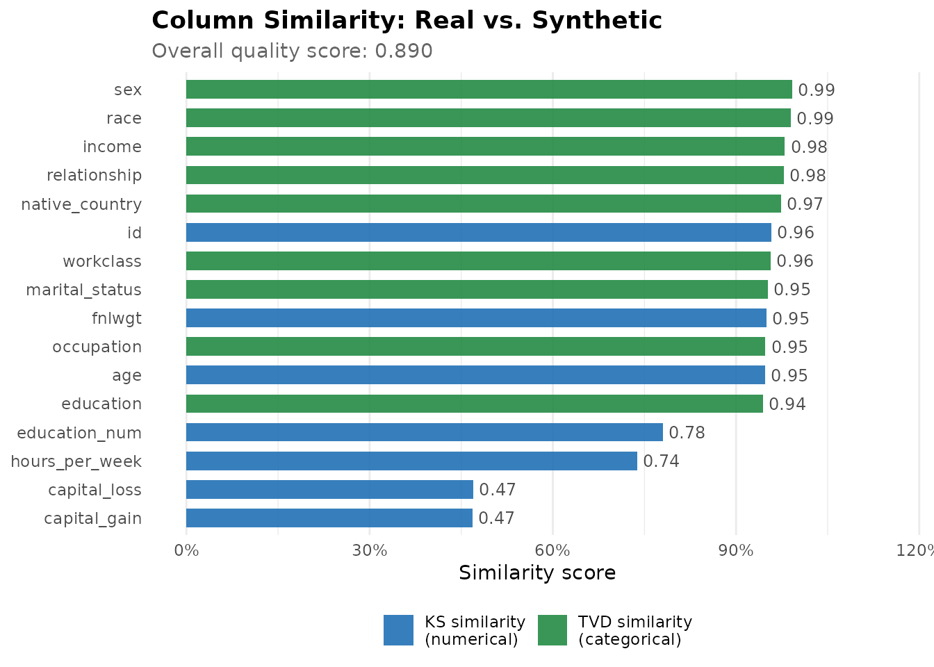
Kolmogorov-Smirnov (KS) similarity measures the maximum absolute difference between the empirical CDFs of a numerical column in the real and synthetic datasets, scored 0–1 (1 = identical distributions). Total variation distance (TVD) similarity is the analogous measure for categorical columns: it computes the maximum difference in probability mass between the real and synthetic frequency distributions, on the same scale. Together they form the Column Shapes property.

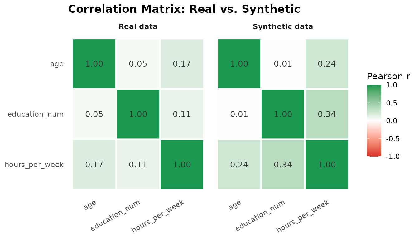
The Column Pair Trends property captures pairwise dependence: correlation similarity (1 - |corr_real - corr_syn| / 2, averaged over numerical pairs) and contingency similarity (1 - TVD between the joint distributions of each categorical pair). Inspect them with correlation_similarity() and contingency_similarity() — each returns per-pair scores alongside the mean.

Correlation structure

The Gaussian copula’s primary purpose is to preserve inter-column correlation; the heatmaps below compare the Pearson correlation matrices for the numerical columns in real and synthetic data.

num_cols <- c("age", "education_num", "hours_per_week")

cor_real <- round(cor(adult_income[, num_cols], use = "complete.obs"), 3)
cor_syn  <- round(cor(synth[, num_cols],        use = "complete.obs"), 3)

mat_to_long <- function(mat, source) {
  nms <- colnames(mat)
  data.frame(
    var1   = rep(nms, each  = length(nms)),
    var2   = rep(nms, times = length(nms)),
    value  = as.vector(mat),
    source = source,
    stringsAsFactors = FALSE
  )
}

cor_long <- rbind(
  mat_to_long(cor_real, "Real data"),
  mat_to_long(cor_syn,  "Synthetic data")
)
cor_long$var1 <- factor(cor_long$var1, levels = rev(num_cols))
cor_long$var2 <- factor(cor_long$var2, levels = num_cols)

ggplot2::ggplot(cor_long, ggplot2::aes(var2, var1, fill = value)) +
  ggplot2::geom_tile(colour = "white", linewidth = 0.8) +
  ggplot2::geom_text(
    ggplot2::aes(label = sprintf("%.2f", value)),
    size = 3.5, colour = "grey20"
  ) +
  ggplot2::facet_wrap(~source) +
  ggplot2::scale_fill_gradient2(
    low      = "#d73027",
    mid      = "white",
    high     = "#1a9850",
    midpoint = 0,
    limits   = c(-1, 1),
    name     = "Pearson r"
  ) +
  ggplot2::labs(
    title = "Correlation Matrix: Real vs. Synthetic",
    x = NULL, y = NULL
  ) +
  ggplot2::theme_minimal(base_size = 11) +
  ggplot2::theme(
    axis.text.x     = ggplot2::element_text(angle = 30, hjust = 1),
    strip.text      = ggplot2::element_text(face = "bold"),
    legend.position = "right",
    plot.title      = ggplot2::element_text(face = "bold"),
    panel.grid      = ggplot2::element_blank()
  )

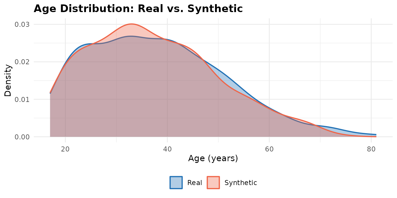
Marginal distributions

Overlaid density curves compare synthetic and real marginals directly.

age_data <- rbind(
  data.frame(value = adult_income$age, source = "Real"),
  data.frame(value = synth$age,        source = "Synthetic")
)

ggplot2::ggplot(age_data, ggplot2::aes(x = value, fill = source, colour = source)) +
  ggplot2::geom_density(alpha = 0.35, linewidth = 0.7) +
  ggplot2::scale_fill_manual(values   = c("Real" = "#2171b5", "Synthetic" = "#ef6548")) +
  ggplot2::scale_colour_manual(values = c("Real" = "#2171b5", "Synthetic" = "#ef6548")) +
  ggplot2::labs(
    title  = "Age Distribution: Real vs. Synthetic",
    x      = "Age (years)", y = "Density",
    fill   = NULL, colour = NULL
  ) +
  ggplot2::theme_minimal(base_size = 11) +
  ggplot2::theme(
    legend.position = "bottom",
    plot.title      = ggplot2::element_text(face = "bold")
  )

income_real  <- as.data.frame(table(adult_income$income) / nrow(adult_income))
income_synth <- as.data.frame(table(synth$income)        / nrow(synth))
names(income_real)  <- c("category", "proportion")
names(income_synth) <- c("category", "proportion")
income_real$source  <- "Real"
income_synth$source <- "Synthetic"
income_data <- rbind(income_real, income_synth)

ggplot2::ggplot(
  income_data,
  ggplot2::aes(x = category, y = proportion, fill = source)
) +
  ggplot2::geom_col(position = "dodge", width = 0.55, alpha = 0.9) +
  ggplot2::scale_y_continuous(labels = scales::percent_format(accuracy = 1)) +
  ggplot2::scale_fill_manual(values = c("Real" = "#2171b5", "Synthetic" = "#ef6548")) +
  ggplot2::labs(
    title = "Income Category: Real vs. Synthetic",
    x = NULL, y = "Proportion", fill = NULL
  ) +
  ggplot2::theme_minimal(base_size = 11) +
  ggplot2::theme(
    legend.position = "bottom",
    plot.title      = ggplot2::element_text(face = "bold")
  )

Diagnostic checks

Where the quality report measures how closely synthetic data resembles the real data, the diagnostic report checks whether it is structurally valid — independent of distributional fidelity. It verifies three things: that numerical values fall within the observed range (boundary adherence), that categorical values use only seen categories (category adherence), and that any primary key is unique and complete (key uniqueness). The package rolls these into a Data Validity score alongside a Data Structure score for column coverage.

dr <- diagnostic_report(adult_income, synth, meta)
print(dr)
#> == rsdv Diagnostic Report ==
#> 
#> Data Validity (per column):
#>   id                   boundary adherence   1.000
#>   age                  boundary adherence   1.000
#>   fnlwgt               boundary adherence   1.000
#>   education_num        boundary adherence   1.000
#>   capital_gain         boundary adherence   1.000
#>   capital_loss         boundary adherence   1.000
#>   hours_per_week       boundary adherence   1.000
#>   workclass            category adherence   1.000
#>   education            category adherence   1.000
#>   marital_status       category adherence   1.000
#>   occupation           category adherence   1.000
#>   relationship         category adherence   1.000
#>   race                 category adherence   1.000
#>   sex                  category adherence   1.000
#>   native_country       category adherence   1.000
#>   income               category adherence   1.000
#> 
#> Data Validity score:   1.000
#> Data Structure score:  1.000
#> 
#> Overall Score:         1.000

Trust the quality scores only after the diagnostic passes (scores at or near 1) — structurally invalid data cannot be high-quality, no matter how the marginals look.

---

Evaluating Privacy

pr <- privacy_report(adult_income, synth)
print(pr)
#> == rsdv Privacy Report ==
#> 
#> NNDR Score (higher = more private):  0.990

score_val <- pr$nndr_score

zones <- data.frame(
  xmin  = c(0,    0.25, 0.50, 0.75),
  xmax  = c(0.25, 0.50, 0.75, 1.00),
  ymid  = 0.5,
  label = c("High risk", "Moderate", "Good", "Excellent"),
  fill  = c("#d73027",   "#fee090",  "#a6d96a", "#1a9850"),
  stringsAsFactors = FALSE
)

ggplot2::ggplot() +
  ggplot2::geom_rect(
    data = zones,
    ggplot2::aes(xmin = xmin, xmax = xmax, ymin = 0, ymax = 1, fill = fill),
    alpha = 0.35
  ) +
  ggplot2::geom_text(
    data = zones,
    ggplot2::aes(x = (xmin + xmax) / 2, y = 0.15, label = label),
    size = 3, colour = "grey30"
  ) +
  ggplot2::geom_segment(
    data = data.frame(x = score_val),
    ggplot2::aes(x = x, xend = x, y = 0, yend = 1),
    colour = "black", linewidth = 1.6
  ) +
  ggplot2::geom_label(
    data = data.frame(x = score_val),
    ggplot2::aes(x = x, y = 0.72,
                 label = sprintf("NNDR = %.3f", x)),
    hjust = -0.08, size = 3.8, fontface = "bold",
    fill = "white", label.size = 0
  ) +
  ggplot2::scale_fill_identity() +
  ggplot2::scale_x_continuous(
    limits = c(0, 1),
    labels = scales::percent_format(accuracy = 1),
    expand = c(0, 0)
  ) +
  ggplot2::labs(
    title    = "Privacy Score: Nearest-Neighbour Distance Ratio (NNDR)",
    subtitle = "Higher score = lower re-identification risk",
    x = "NNDR score", y = NULL
  ) +
  ggplot2::theme_minimal(base_size = 11) +
  ggplot2::theme(
    axis.text.y      = ggplot2::element_blank(),
    axis.ticks.y     = ggplot2::element_blank(),
    panel.grid       = ggplot2::element_blank(),
    plot.title       = ggplot2::element_text(face = "bold"),
    plot.subtitle    = ggplot2::element_text(colour = "grey40")
  )

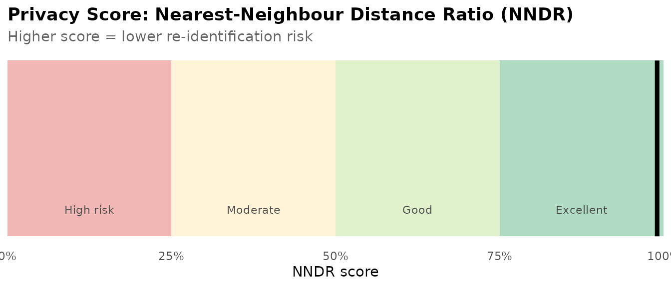
The Nearest-Neighbour Distance Ratio (NNDR) compares each synthetic row’s distance to its nearest real neighbour against its distance to its second-nearest. A high NNDR (near 1) means no synthetic row is suspiciously close to any one real record — the hallmark of low re-identification risk. A score below 0.5 suggests the synthesis is memorising real rows rather than learning the distribution.

By default nndr() z-scores each numerical column using the real-data mean and standard deviation before computing the Euclidean distance. Without this step, a single large-scale column — income in dollars, for instance — dominates the distance and the score moves with units rather than similarity. Pass normalize = FALSE to opt out.

For attribute disclosure risk — estimating how easily a known set of background variables can be used to infer a sensitive value — use attribute_disclosure_risk():

adr <- attribute_disclosure_risk(
  real          = adult_income,
  synthetic     = synth,
  sensitive_col = "income",
  known_cols    = "age"
)
cat("Attribute disclosure risk (income given age):", round(adr, 3), "\n")
#> Attribute disclosure risk (income given age): 0.636

---

Adding Constraints

Constraints enforce domain-knowledge rules the copula model alone will not guarantee. The system uses rejection sampling: rsdv discards rows that fail any constraint and draws replacements until n valid rows are collected.

meta_constrained <- meta |>
  add_constraint(
    inequality_constraint("education_num", "hours_per_week", type = "lt")
  )

syn_c   <- gaussian_copula_synthesizer(meta_constrained) |> fit(adult_income)
synth_c <- sample(syn_c, n = 500)

# Verify: education_num < hours_per_week in all rows — should return TRUE
all(synth_c$education_num < synth_c$hours_per_week)
#> [1] TRUE

Available constraint types:

Function	Condition enforced
equality_constraint(a, b, tolerance = 0)	a == b row-wise (or abs(a - b) <= tolerance for numerics when tolerance > 0)
inequality_constraint(a, b, type)	a < b, a <= b, a > b, or a >= b
fixed_combinations_constraint(cols, ref)	Only combinations present in ref are permitted
custom_constraint(fn, vectorized = FALSE)	Arbitrary predicate; with vectorized = TRUE, fn is called once on the whole data frame for a substantial speedup

For continuous numerical columns, exact == almost never holds — use the tolerance argument on equality_constraint() (or a tight band of inequality_constraint()s). Rows containing NA fail equality and inequality checks, so the sampler rejects them instead of producing phantom NA rows.

---

Handling Missing Data

What rsdv does by default

When a column contains NA values in the training data, rsdv records the empirical missingness rate and reproduces it in synthetic output by randomly assigning NA to the same proportion of rows at sampling time. The copula is fitted on complete cases only.

This behaviour is appropriate when data are missing completely at random (MCAR) — that is, when the probability that a value is missing is unrelated to the value itself or to any other observed variable. Survey item non-response caused by form layout errors, laboratory equipment failures on random days, or random attrition in a longitudinal study are plausible examples.

When to pre-impute

Two mechanisms produce missingness patterns that MCAR-based synthesis handles poorly:

Missing at random (MAR): the probability of missingness depends on other observed variables. Income non-response that is higher among older respondents, or laboratory values missing because a clinician ordered fewer tests for healthier patients, are MAR. The copula captures conditional distributions among observed values correctly but does not model the relationship between missingness and its predictors.

Missing not at random (MNAR): the probability of missingness depends on the unobserved value itself. High earners declining to report income, or patients with the worst prognosis dropping out of a trial, are MNAR. No synthesis method fully recovers from MNAR without auxiliary information.

For MAR data, pre-imputation before synthesis is recommended:

# Pre-impute systematically missing data before synthesis
library(mice)
imputed <- complete(mice(your_data, m = 1, printFlag = FALSE))
syn <- gaussian_copula_synthesizer(meta) |> fit(imputed) |> sample(n = 500)

The missRanger package provides a fast random forest–based alternative suitable for larger datasets.

---

Considerations and Caveats

Sample size. Gaussian copula estimation is stable for datasets with at least a few dozen rows per numerical dimension. The package uses Kendall’s τ–based correlation estimation, which is more robust than maximum likelihood for small samples, but correlation estimates become noisy when the number of rows is small relative to the number of numerical columns. A dataset with 3 numerical columns and 100 rows is well-conditioned; the same 100 rows with 15 numerical columns is not.

When a categorical column has more unique levels than the synthetic sample size, some levels will be absent from the synthetic output — expected sampling behaviour. If level coverage matters, increase n or aggregate rare levels before synthesis.

Unsupported column types. Columns typed as "id" or "datetime" are excluded from synthesis and will not appear in synthetic output. fit() emits a warning listing excluded columns. A common workaround is to convert date variables to numeric before synthesis and convert them back afterward.

The Gaussian copula assumes elliptical (roughly symmetric) dependence. It will underrepresent tail dependence — situations where extreme values in one variable coincide with extreme values in another, which is common in financial returns, insurance claims, and natural disaster data. For heavy-tailed dependence structures, a t-copula or vine copula extension is more appropriate.

Categorical and boolean columns are embedded in the copula via their cumulative-frequency intervals, so associations between categorical columns — and between categorical and numerical columns — are preserved. Because the embedding is rank-based and the latent dependence is Gaussian, very fine-grained or strongly non-monotone categorical associations may be modeled only approximately; the contingency_similarity() metric reports how well categorical pair associations are reproduced.

Synthesis reduces re-identification risk but does not eliminate it. The NNDR and attribute disclosure risk metrics in rsdv provide quantitative estimates of residual risk. Use the built-in privacy report as a starting point, and consult your institution’s data governance office for a formal privacy impact assessment in regulated environments.

---

Citation

If you use rsdv in published research, please cite the package:

@Manual{Venkitasubramanian2026rsdv,
  title  = {{rsdv}: Synthetic Tabular Data Generation with Gaussian Copulas},
  author = {Venkitasubramanian, Kailas},
  year   = {2026},
  note   = {R package version 0.2.0},
  url    = {https://CRAN.R-project.org/package=rsdv},
  doi    = {10.32614/CRAN.package.rsdv}
}

You can also retrieve the citation from within R:

citation("rsdv")

Contact and feedback: Questions, bug reports, and feature requests are welcome at kvenkita@charlotte.edu or via the GitHub issue tracker.

Copyright © 2026 Kailas Venkitasubramanian. Released under the MIT License.

---

References

Hofert, M., Kojadinovic, I., Mächler, M., and Yan, J. (2018). Elements of Copula Modeling with R. Springer. (See also: R package copula, https://cran.r-project.org/package=copula.)

Nowok, B., Raab, G. M., and Dibben, C. (2016). synthpop: Bespoke creation of synthetic data in R. Journal of Statistical Software, 74(11), 1–26. DOI:10.18637/jss.v074.i11. https://www.jstatsoft.org/article/view/v074i11.

Patki, N., Wedge, R., and Veeramachaneni, K. (2016). The synthetic data vault. IEEE International Symposium on Data Science and Advanced Analytics (DSAA), 399–410. DOI:10.1109/DSAA.2016.49. https://ieeexplore.ieee.org/document/7796926/.

Raab, G. M., Nowok, B., and Dibben, C. (2024). Practical privacy metrics for synthetic data. arXiv:2406.16826. https://arxiv.org/abs/2406.16826.

Sklar, A. (1959). Fonctions de répartition à n dimensions et leurs marges. Publications de l’Institut de Statistique de l’Université de Paris, 8, 229–231.

Templ, M., Kowarik, A., and Meindl, B. (2015). Statistical disclosure control for micro-data using the R package sdcMicro. Journal of Statistical Software, 67(4), 1–36. DOI:10.18637/jss.v067.i04.

Tomilina, G., Mazo, G., and Jaffrézic, F. (2024). A semi-parametric Gaussian copula model for heterogeneous network inference: an application to multi-omics data. HAL preprint hal-04847648. https://hal.inrae.fr/hal-04847648.

Watson, D. S., Blesch, K., Kapar, J., and Wright, M. N. (2023). Adversarial random forests for density estimation and generative modeling. Proceedings of the 26th International Conference on Artificial Intelligence and Statistics (AISTATS), PMLR 206:5357–5375. https://proceedings.mlr.press/v206/watson23a.html.