A primer: doubly robust LATE estimation, from intuition to practice

This primer explains, with as little formalism as possible, what the estimators in drlate do and when you would want them. It is a companion to two papers by Słoczyński, Uysal, and Wooldridge: “Doubly Robust Estimation of Local Average Treatment Effects Using Inverse Probability Weighted Regression Adjustment” (2022, arXiv:2208.01300), whose estimators the authors’ Stata command drlate implements, and “Abadie’s Kappa and Weighting Estimators of the Local Average Treatment Effect” (2025, JBES), whose estimator menu their command kappalate implements. This package implements both papers behind one interface. Along the way the primer demonstrates every tool in the package: estimation, the weighting-estimator menu, diagnostics, weak-instrument-robust inference, the bootstrap, the estimator comparison, and the doubly robust Hausman test.

1. The problem: a treatment people choose

Suppose you want to know the effect of a treatment $D$ (a job training program, military service, a 401(k) plan) on an outcome $Y$ (wages, savings). People choose whether to take the treatment, and the ones who take it differ from the ones who don’t in ways you can’t fully observe. Comparing treated and untreated outcomes, even with regression controls, confounds the effect of the treatment with the effect of being the kind of person who takes it.

The classic escape is an instrument $Z$ : a binary variable that shifts the likelihood of treatment but has no direct channel to the outcome. Draft lottery numbers, distance to a college, randomized encouragement to participate — all push some people into treatment without otherwise touching their outcomes.

Imbens and Angrist (1994) showed what an instrument can and cannot give you. It cannot reveal the effect of treatment for everyone. It identifies the effect for compliers — the people whose treatment status is actually moved by the instrument. That quantity is the local average treatment effect:

$\text{LATE} \;=\; \frac{\;\text{effect of } Z \text{ on } Y\;} {\;\text{effect of } Z \text{ on } D\;}$

The numerator is the intent-to-treat effect; the denominator is the first stage (the share of compliers). With no covariates this ratio is the Wald estimator, and it is exactly what two-stage least squares computes.

Why covariates enter

Real instruments are rarely as clean as a lottery. Distance to college is exogenous given family background and region; a draft lottery is clean, but conditioning on covariates still buys precision. So in practice you need the instrument to be as-good-as-random conditional on covariates $X$ , and then both the numerator and the denominator above become covariate-adjusted contrasts. How exactly to adjust them is the entire subject of the 2022 paper and this package.

2. The four core estimators in one picture

All estimators in drlate build the same ratio; they differ only in how each piece is adjusted for $X$ . This section covers the four regression-and-weighting strategies from the 2022 paper; a second family, the Abadie-kappa weighting menu from the 2025 paper, appears in Section 6. Each piece is an “effect of $Z$ on something”, a problem formally identical to estimating an average treatment effect of $Z$ under unconfoundedness, so the familiar treatment-effects toolbox applies:

`method`	How it adjusts	Needs correct…
`"ra"`	Regression adjustment: model $Y$ (and $D$ ) given $X$ in each instrument arm; average the predictions.	outcome/treatment models
`"ipw"`	Inverse probability weighting: model the instrument propensity score $p(X) = \Pr(Z=1 \mid X)$ ; reweight raw means by $1/p$ and $1/(1-p)$ .	propensity score
`"aipw"`	Augmented IPW: regression adjustment plus an IPW correction term.	either one
`"ipwra"`	IPW regression adjustment: fit the outcome/treatment regressions weighted by the inverse propensity score.	either one

The last two are doubly robust (DR): they are consistent if the propensity score model or the regression models are right — you get two chances instead of one.

Why the paper (and the package default) prefers IPWRA

AIPW achieves double robustness by adding a correction term, and that sum can wander outside the logical range of the outcome — a predicted probability of 1.3, a negative count. IPWRA achieves it by reweighting a quasi-likelihood regression, so as long as you choose a sensible family (logit for binary outcomes, Poisson for counts), fitted values stay in range by construction. Hence IPWRA’s appealing small-sample behavior in the paper’s simulations, and its place as the package default.

A second practical lesson from the paper concerns normalization. Raw IPW weights $Z_i/\hat p(X_i)$ need not average to one in a sample; if a few observations have small estimated propensity scores, unnormalized estimators can be erratic. Normalizing the weights to sum to one (the Hájek construction) fixes this and costs nothing, so normalized = TRUE is the default. It matters only for "ipw" and "aipw"; IPWRA is normalized by construction.

3. A worked example

drlate_sim is a simulated dataset built so that the truth is known: a binary instrument rsncode, a binary treatment nvstat with two-sided noncompliance (60% compliers), and a continuous outcome lwage. The true effect for compliers is 0.5. The design plants two traps for the naive approaches: the treatment is endogenous (people who always take it have higher baseline outcomes), and the instrument is not unconditionally random (the probability of rsncode = 1 rises with age and education, which also shift the outcome).

library(drlate)
data(drlate_sim)
str(drlate_sim)
#> 'data.frame':    2000 obs. of  7 variables:
#>  $ lwage  : num  1.892 -1.625 -0.484 0.92 -0.392 ...
#>  $ kwage  : num  2.575 0.444 0.785 1.584 0.822 ...
#>  $ hijob  : int  1 0 0 0 0 0 0 0 1 1 ...
#>  $ nvstat : int  0 0 0 1 0 1 0 1 0 1 ...
#>  $ rsncode: int  1 0 1 1 0 1 0 1 0 1 ...
#>  $ age    : num  37 12 31 27 33 33 23 29 37 51 ...
#>  $ educ   : Factor w/ 3 levels "hs","college",..: 1 1 1 2 2 2 1 1 1 1 ...

The naive answers fail

Comparing treated to untreated (even though this is “just a regression”):

coef(lm(lwage ~ nvstat + age + educ, drlate_sim))["nvstat"]
#>    nvstat 
#> 0.8425038

Biased upward — always-takers are different people. The raw Wald ratio ignores that the instrument favors older, more educated workers:

with(drlate_sim,
     (mean(lwage[rsncode == 1]) - mean(lwage[rsncode == 0])) /
     (mean(nvstat[rsncode == 1]) - mean(nvstat[rsncode == 0])))
#> [1] 1.045469

Twice the truth.

The drlate answer

Three formulas, one per model: the outcome model, the treatment model, and the instrument propensity score model.

fit <- drlate(outcome    = lwage   ~ age + educ,
              treatment  = nvstat  ~ age + educ,
              instrument = rsncode ~ age + educ,
              data = drlate_sim)
summary(fit)
#> 
#> Local average treatment effect
#> Number of obs    : 2,000
#> Estimator        : IPWRA
#> Outcome model    : linear
#> Treatment model  : logit
#> Instrument model : logit (MLE)
#> 
#>              Estimate Std. Error z value   Pr(>|z|) [95% conf. interval]
#> LATE: D on Y   0.4705    0.07915   5.944  2.786e-09     0.3153    0.6256
#> ATE: Z on Y    0.2845    0.05043   5.642  1.679e-08     0.1857    0.3834
#> ATE: Z on D    0.6048    0.01837  32.929 8.326e-238     0.5688    0.6408
#> 
#> First stage (Z on D): z = 32.93 (z^2 ~ first-stage F = 1084)

Read the three rows bottom-up:

ATE: Z on D — the first stage: the instrument moves the treatment probability by about 0.60 (the complier share).
ATE: Z on Y — the intent-to-treat effect of the instrument on the outcome.
LATE: D on Y — their ratio, the causal effect for compliers. The 95% interval comfortably covers the true 0.5.

The final line reports first-stage strength: with a single binary instrument, the squared z-statistic is the first-stage robust F. Here F ≈ 1084, far above the conventional F = 10 danger threshold, so Wald inference on the ratio is trustworthy. Section 7 shows what the package does when it isn’t.

The standard errors here are not an afterthought: drlate stacks every estimation stage (the propensity score, both outcome regressions, both treatment regressions, and the ratio itself) into one moment system and computes a joint sandwich variance. The uncertainty from estimating the propensity score propagates into the LATE’s standard error, exactly as in the Stata original.

Seeing double robustness work

The DGP has the propensity score and the outcomes both depending on age and educ. Give the estimator a wrong propensity score model (intercept only) but correct regressions — then a wrong outcome model but a correct propensity score:

# Propensity score misspecified; regressions correct
coef(drlate(lwage ~ age + educ, nvstat ~ age + educ, rsncode ~ 1,
            data = drlate_sim))[1]
#> LATE: D on Y 
#>    0.4597253

# Regressions misspecified (intercept only); propensity score correct
coef(drlate(lwage ~ 1, nvstat ~ 1, rsncode ~ age + educ,
            data = drlate_sim))[1]
#> LATE: D on Y 
#>    0.4740516

Either way the estimate stays near 0.5: one correct model is enough. (Misspecify both and no estimator can save you.)

4. Checking the design: diagnostics

An estimate deserves evidence that the design behind it is sound. drlate provides the standard design diagnostics — propensity-score overlap, covariate balance, and the implied weight distribution — together with a formal balance test and a profile of the compliers. The last several mirror the postestimation tools of Stata’s lateffects command.

Overlap

IPW-type estimators divide by $\hat p(X)$ and $1-\hat p(X)$ , so the estimated instrument propensity scores must stay away from 0 and 1. Healthy overlap looks like two well-mixed distributions:

plot(fit, type = "overlap")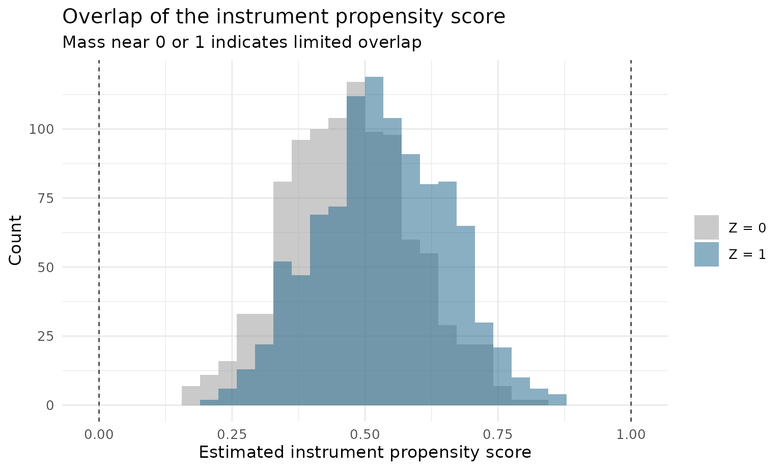

drlate() refuses to estimate if any score breaches [pstolerance, 1 - pstolerance]; set osample = TRUE to get back an indicator of the violating observations instead, so you can inspect them before restricting the sample. Pass geom = "density" to draw the same check as smoothed kernel densities.

Covariate balance

The whole point of weighting by the inverse propensity score is to make the instrument arms comparable on covariates. The love plot shows standardized mean differences before and after weighting — weighted dots inside the conventional ±0.1 band mean the propensity score model is doing its job:

plot(fit, type = "balance")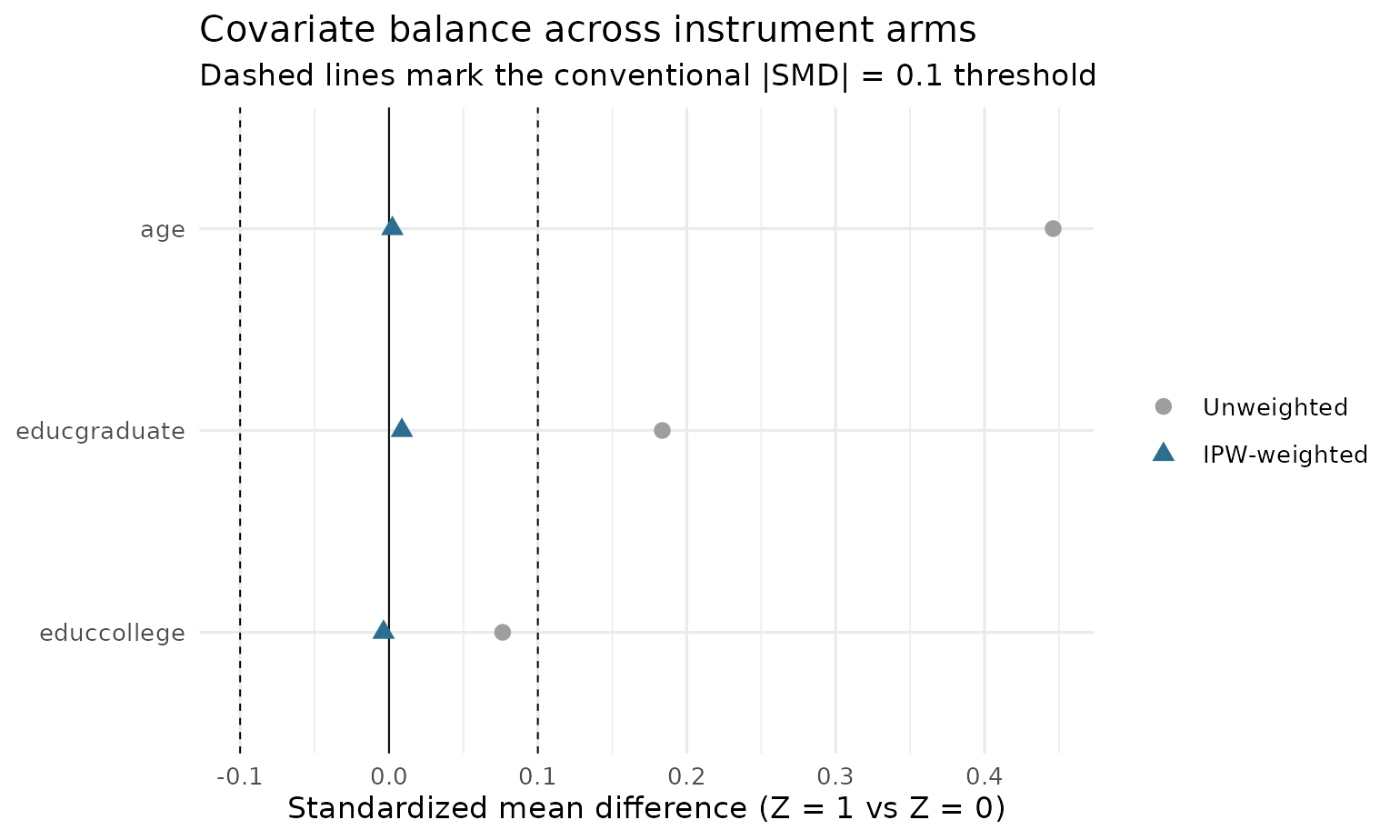

The underlying numbers come from balance():

balance(fit)
#>       variable smd_unweighted smd_weighted
#> 1          age     0.44613912  0.002276611
#> 2  educcollege     0.07633523 -0.003643849
#> 3 educgraduate     0.18356486  0.008657272

age moves from a standardized difference of 0.45 to nearly zero after weighting. Add detail = TRUE for the weighted arm means and variance ratios as well. To see distributions rather than summaries, plot(fit, type = "balance_density") overlays each covariate’s kernel density across the instrument arms, raw versus weighted — a balanced covariate has arm densities that coincide in the weighted panel:

plot(fit, type = "balance_density", var = "age")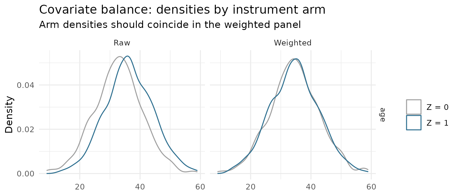

Weight distributions

A few enormous weights mean a few observations dominate the estimate — the classic symptom of thin overlap:

plot(fit, type = "weights")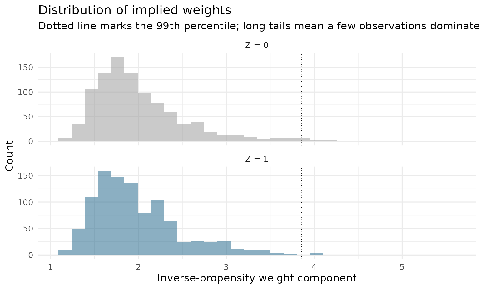

A formal balance test

The love plot is an eyeball test; balance_test() is the formal one. It implements the Imai and Ratkovic (2014) overidentification test of whether the propensity-score model balances the covariates. A small p-value is evidence that the score is misspecified:

balance_test(fit)
#> Imai-Ratkovic covariate-balance test (overidentification)
#> 
#>   Hansen J = 3.0473   df = 4   p-value = 0.5499
#>   Instrument propensity score: logit (n = 2000)
#> 
#>   H0: the propensity-score model balances the covariates.

Profiling the compliers

Because the LATE is an effect for compliers, it helps to know how they differ from the population. complier_means() compares each covariate’s overall mean with its mean among compliers, the latter weighted by Abadie’s $\kappa$ :

complier_means(fit)
#>       variable population_mean complier_mean   difference
#> 1          age         34.5560    34.3303393 -0.225660695
#> 2  educcollege          0.3615     0.3590211 -0.002478943
#> 3 educgraduate          0.1395     0.1431700  0.003670025

The weights themselves are available through kappa_weights(fit) for building other complier summaries.

5. Choosing models and options

Outcome and treatment families

The treatment and the outcome may each be continuous, binary, a count, or a fraction; choose families so fitted values respect the response’s range — the heart of the IPWRA recommendation:

# Binary outcome: logit keeps fitted probabilities in [0, 1]
coef(drlate(hijob ~ age + educ, nvstat ~ age + educ, rsncode ~ age + educ,
            data = drlate_sim, omodel = "logit"))
#> LATE: D on Y  ATE: Z on Y  ATE: Z on D 
#>    0.1742853    0.1054104    0.6048151

# Positive outcome: Poisson (quasi-likelihood; no distributional claim)
coef(drlate(kwage ~ age + educ, nvstat ~ age + educ, rsncode ~ age + educ,
            data = drlate_sim, omodel = "poisson"))
#> LATE: D on Y  ATE: Z on Y  ATE: Z on D 
#>    0.6088370    0.3682338    0.6048151

Binary outcomes also accept omodel = "probit", and a response confined to the unit interval — a proportion or rate — uses omodel = "flogit" or "fprobit". The fractional families share all estimation with "logit" / "probit" and only relax the response to [0, 1], matching the Stata lateffects omodel options.

Instrument propensity score flavors

Beyond logit MLE, two estimators tailor the propensity score to its job in the weights:

ivmodel = "cbps" — covariate balancing (Imai and Ratkovic 2014): chooses the logit coefficients so the inverse-probability weights exactly balance the covariates between instrument arms.
ivmodel = "ipt" — inverse probability tilting (Graham, Pinto, and Egel 2012): fits a separate tilted score per arm; the resulting weights are exactly normalized by construction.
ivmodel = "probit" — probit maximum likelihood, mirroring kappalate’s zmodel(probit); available for the weighting estimators ("ipw" and the kappa methods of Section 6).

coef(drlate(lwage ~ age + educ, nvstat ~ age + educ, rsncode ~ age + educ,
            data = drlate_sim, ivmodel = "ipt"))[1]
#> LATE: D on Y 
#>    0.4706598

# probit propensity score with a weighting estimator (Section 6)
coef(drlate(lwage ~ 1, nvstat ~ 1, rsncode ~ age + educ,
            data = drlate_sim, method = "kappa10",
            ivmodel = "probit"))[1]
#> LATE: D on Y 
#>    0.4738596

LATT: the effect for treated compliers

estimand = "latt" reweights everything toward the treated population — “among those who took the treatment, what did it do?”:

coef(drlate(lwage ~ age + educ, nvstat ~ age + educ, rsncode ~ age + educ,
            data = drlate_sim, estimand = "latt"))
#> LATT: D on Y  ATT: Z on Y  ATT: Z on D 
#>    0.4725042    0.2844545    0.6020148

Weights (weights =) and clustered standard errors (cluster =) are available everywhere.

The companion paper Słoczyński, Uysal, and Wooldridge (2025) studies the family of pure weighting estimators of the LATE motivated by Abadie’s (2003) kappa theorem. These use only the instrument propensity score — no outcome or treatment regressions — and differ in which kappa weights they use and whether the weights are normalized. drlate implements the full menu of the authors’ Stata command kappalate:

`method`	kappalate name	Weighting
`"kappa"`	`tau_a`	unnormalized Abadie kappa
`"ipw"`, `normalized = FALSE`	`tau_a,1`	unnormalized, treated-arm
`"kappa0"`	`tau_a,0`	unnormalized, untreated-arm
`"kappa10"`	`tau_a,10`	normalized Abadie kappa
`"ipw"` (default normalized)	`tau_u`	normalized (Hájek)

Because the kappa methods carry no outcome or treatment model, the first two formulas must be intercept-only, and that makes the whole menu a like-for-like comparison (every row adjusts for covariates only through the instrument propensity score):

cmp_w <- drlate_compare(lwage ~ 1, nvstat ~ 1, rsncode ~ age + educ,
                        data = drlate_sim,
                        methods = c("ipw", "kappa", "kappa0", "kappa10"))
cmp_w
#> Estimator comparison (LATE)
#> 
#>  estimator estimate     se           95% CI
#>  ipw (nrm)   0.4741 0.0793 [0.3187, 0.6295]
#>      kappa   0.4731 0.0800 [0.3164, 0.6298]
#>     kappa0   0.4733 0.0803 [0.3159, 0.6306]
#>    kappa10   0.4740 0.0793 [0.3186, 0.6294]

All four sit on top of each other here — a healthy design. The paper’s main practical lesson is which of these to trust when they disagree: the normalized estimators (tau_u, i.e. method = "ipw", and tau_a,10), because the unnormalized variants are sensitive to the location and scale of the outcome. You can see that sensitivity directly. Shift the outcome by a constant, which should not change a treatment effect:

d_shift <- transform(drlate_sim, lwage = lwage + 100)
rbind(
  kappa10 = c(original = coef(drlate(lwage ~ 1, nvstat ~ 1,
                                     rsncode ~ age + educ,
                                     data = drlate_sim,
                                     method = "kappa10"))[[1]],
              shifted = coef(drlate(lwage ~ 1, nvstat ~ 1,
                                    rsncode ~ age + educ,
                                    data = d_shift,
                                    method = "kappa10"))[[1]]),
  kappa   = c(original = coef(drlate(lwage ~ 1, nvstat ~ 1,
                                     rsncode ~ age + educ,
                                     data = drlate_sim,
                                     method = "kappa"))[[1]],
              shifted = coef(drlate(lwage ~ 1, nvstat ~ 1,
                                    rsncode ~ age + educ,
                                    data = d_shift,
                                    method = "kappa"))[[1]])
)
#>          original   shifted
#> kappa10 0.4740434 0.4740434
#> kappa   0.4731112 0.4242734

The normalized kappa10 is exactly invariant; the unnormalized kappa moves. (The package prints each estimator’s kappalate name so the mapping above is always visible in the output.)

Unlike the Stata command, all of drlate’s inference machinery applies to the kappa menu: cluster-robust standard errors, sampling weights, the bootstrap, and Fieller confidence sets for "kappa" and "kappa0" ("kappa10" is a difference of two ratios, for which no Fieller pivot exists, so use the bootstrap there).

7. When the instrument is weak: Fieller confidence sets

The LATE is a ratio, and ratios with imprecise denominators behave badly: the usual (delta-method) confidence interval can have far-from-nominal coverage when the first stage is weak. The package watches for this: whenever the first-stage F drops below 10, the printout flags it and shows a Fieller confidence set alongside.

The Fieller set inverts the test of $H_0:\ \text{num} - t \cdot \text{denom} = 0$ using the joint covariance of the numerator and the denominator (which the stacked moment system provides). Unlike the Wald interval, it keeps its promised asymptotic coverage no matter how weak the instrument — at the honest price that it may be unbounded when the data barely identify the ratio.

Watch it engage on a deliberately broken design (instrument shuffled at random in a small subsample, so the true first stage is zero):

set.seed(42)
d_weak <- drlate_sim[1:300, ]
d_weak$zweak <- sample(d_weak$rsncode)
fit_weak <- drlate(lwage ~ age, nvstat ~ age, zweak ~ age, data = d_weak)
print(fit_weak)
#> 
#> Local average treatment effect
#> Number of obs    : 300
#> Estimator        : IPWRA
#> Outcome model    : linear
#> Treatment model  : logit
#> Instrument model : logit (MLE)
#> 
#>               Estimate Std. Error z value Pr(>|z|) [95% conf. interval]
#> LATE: D on Y 13.662047  118.10943  0.1157   0.9079  -217.8282  245.1523
#> ATE: Z on Y  -0.087409    0.12389 -0.7055   0.4805    -0.3302    0.1554
#> ATE: Z on D  -0.006398    0.05692 -0.1124   0.9105    -0.1180    0.1052
#> 
#> First stage (Z on D): z = -0.1124 (z^2 ~ first-stage F = 0.0126)  [weak: Wald inference on the ratio may be unreliable]
#> Fieller 95% confidence set for the late: (-Inf, Inf) - the first stage is uninformative

The Fieller set is available on demand for any fit:

confint(fit, method = "fieller")     # strong instrument: ~ Wald interval
#> Fieller 95% confidence set for LATE: D on Y:
#>   [0.3131, 0.6239]

In the package’s Monte Carlo validation, under a very weak first stage (about 4% compliers) the Fieller set covered the true LATE 95.7% of the time — reporting an unbounded set in roughly 40% of replications, the statistically honest answer — while the Wald interval over-covered at 99.3%, conveying a precision it did not have.

8. Bootstrap inference

The paper notes that inference is straightforward “both analytically and using the nonparametric bootstrap.” The analytic sandwich is the default; the bootstrap re-runs the entire estimation pipeline (including the propensity score) on each resample:

fit_boot <- drlate(lwage ~ age + educ, nvstat ~ age + educ,
                   rsncode ~ age + educ, data = drlate_sim,
                   vcov = "bootstrap", boot_reps = 199, boot_seed = 42)
summary(fit_boot)
#> 
#> Local average treatment effect
#> Number of obs    : 2,000
#> Estimator        : IPWRA
#> Outcome model    : linear
#> Treatment model  : logit
#> Instrument model : logit (MLE)
#> Std. errors      : nonparametric bootstrap (199 of 199 reps)
#> 
#>              Estimate Std. Error z value   Pr(>|z|) [2.5% boot boot 97.5%]
#> LATE: D on Y   0.4705    0.07387   6.369  1.906e-10     0.3240      0.5987
#> ATE: Z on Y    0.2845    0.04748   5.993  2.061e-09     0.1858      0.3746
#> ATE: Z on D    0.6048    0.01852  32.654 7.060e-234     0.5684      0.6417
#> 
#> First stage (Z on D): z = 32.93 (z^2 ~ first-stage F = 1084)

Point estimates are unchanged; standard errors and the confidence intervals (now percentile intervals from the bootstrap distribution) come from the resamples. When cluster is supplied, whole clusters are resampled. Draws that fail — degenerate resamples, overlap violations — are dropped and counted; a non-trivial failure rate is itself a sign of weak identification, in which case prefer the Fieller set.

9. How much does the estimator choice matter?

Referees routinely ask for this table. One call runs all four estimators:

cmp <- drlate_compare(lwage ~ age + educ, nvstat ~ age + educ,
                      rsncode ~ age + educ, data = drlate_sim)
#> method = "ipw": dropping outcome/treatment covariates (weighted means only).
#> method = "ra": dropping instrument covariates (no propensity score).
cmp
#> Estimator comparison (LATE)
#> 
#>   estimator estimate     se           95% CI
#>       ipwra   0.4705 0.0792 [0.3153, 0.6256]
#>   ipw (nrm)   0.4741 0.0793 [0.3187, 0.6295]
#>  aipw (nrm)   0.4702 0.0792 [0.3150, 0.6254]
#>          ra   0.4597 0.0792 [0.3045, 0.6150]
plot(cmp)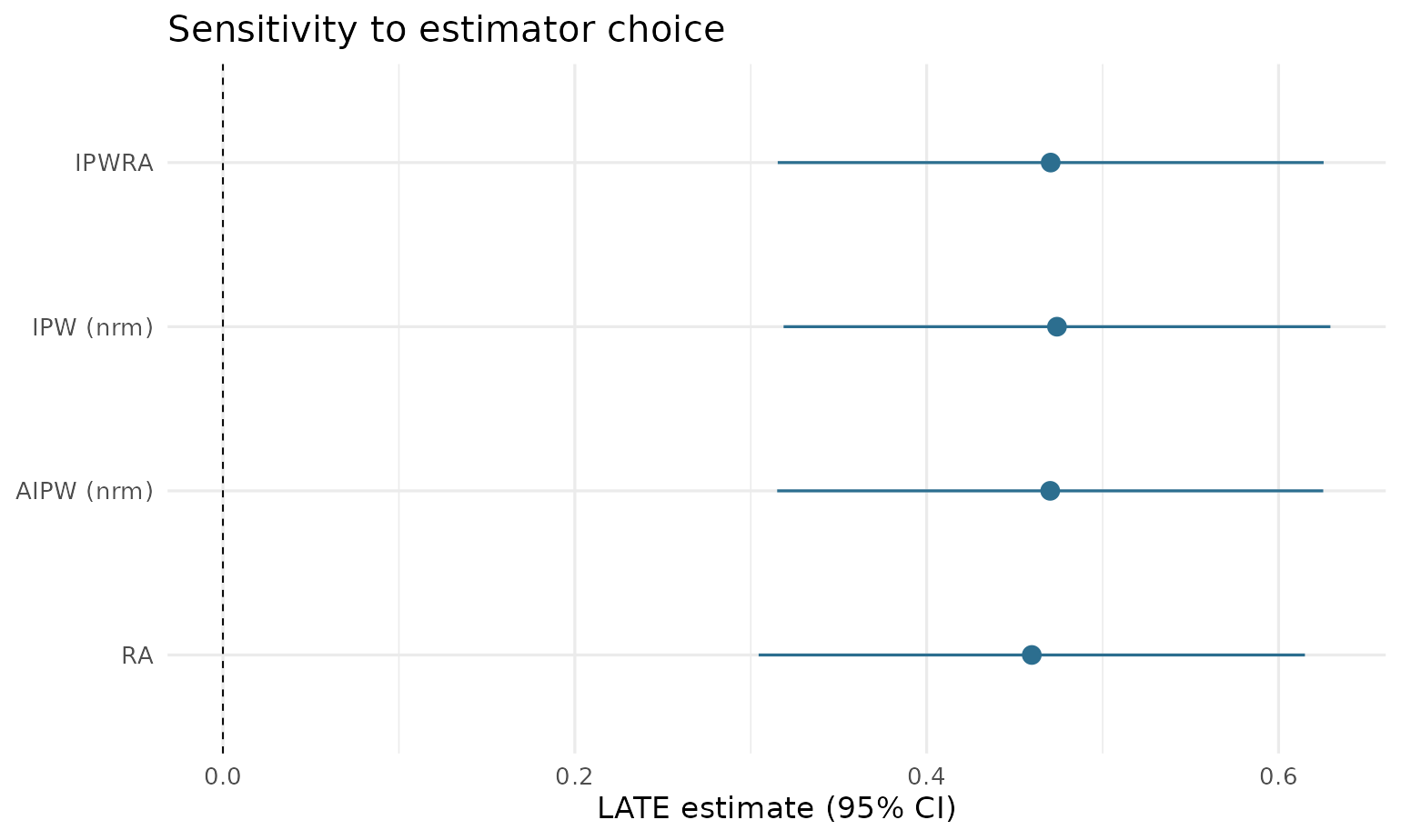

A caveat printed in the documentation bears repeating: IPW carries no outcome/treatment regressions and RA no propensity score, so those rows necessarily use reduced specifications. The IPWRA-vs-AIPW pair is the like-for-like doubly robust comparison. Here all four agree closely, which is what a healthy design looks like.

10. Do you even need the instrument? The DR Hausman test

The 2022 paper’s Section 5 proposes a specification test that the Stata package does not implement. The logic: under one-sided noncompliance (nobody gets the treatment without the instrument), the LATT estimated through the instrument and the ATT estimated assuming the treatment is unconfounded given $X$ target the same parameter — if unconfoundedness holds. So a significant difference between the two doubly robust estimates is evidence against unconfoundedness. Unlike the textbook OLS-vs-IV Hausman test, this comparison survives heterogeneous treatment effects.

The simulated data are built with confounded treatment (always-takers have higher baseline wages), so after imposing one-sided noncompliance the test should — and does — reject:

d_os <- drlate_sim
d_os$nvstat[d_os$rsncode == 0] <- 0L   # impose one-sided noncompliance

dr_hausman(lwage ~ age + educ, nvstat ~ age + educ, rsncode ~ age + educ,
           data = d_os)
#> 
#>  Doubly robust Hausman test of unconfoundedness
#>  (Sloczynski-Uysal-Wooldridge 2022, one-sided noncompliance)
#> 
#> data:  d_os
#> z = -5.7425, p-value = 9.331e-09
#> alternative hypothesis: two.sided
#> sample estimates:
#>    DR LATT     DR ATT difference 
#>  0.3760331  0.6323210 -0.2562878

The unconfoundedness-based ATT (≈ 0.63) is biased upward by exactly the selection the DGP builds in, while the instrument-based LATT (≈ 0.38 in this one-sided subpopulation) is protected. The difference is almost six standard errors from zero. In practice: a rejection says the controls alone do not suffice — you needed the instrument; a non-rejection says the controls may suffice, and the much more precise unconfoundedness-based estimator becomes defensible.

The standard error of the difference is analytic: both estimators’ moment conditions are stacked into one system so their correlation is accounted for — the construction the paper sketches and this package carries out. (In Monte Carlo under a true null the test rejects at 4.7% for a nominal 5% level.)

11. Coming from Stata

Stata	R
`drlate (lwage age_5) (nvstat age_5) (rsncode age_5)`	`drlate(lwage ~ age_5, nvstat ~ age_5, rsncode ~ age_5, data = d)`
`(y x, poisson)`	`omodel = "poisson"`
`(z x, ipt)`	`ivmodel = "ipt"`
`, latt`	`estimand = "latt"`
`, method(aipw) unnrm`	`method = "aipw", normalized = FALSE`
`[pw = w]`	`weights = "w"`
`, vce(cluster id)`	`cluster = "id"`
`i.educ` factor syntax	a `factor()` column in the formula
`kappalate y (d = z) x` (tau_a)	`method = "kappa"`
`kappalate ..., which(all)` (tau_a,0 / tau_a,10)	`method = "kappa0"` / `"kappa10"`
`kappalate ...` (tau_u / tau_a,1)	`method = "ipw"` / `"ipw", normalized = FALSE`
`kappalate ..., zmodel(cbps)`	`ivmodel = "cbps"`
`kappalate ..., zmodel(probit)`	`ivmodel = "probit"`
`lateoverlap`	`plot(type = "overlap")` (with `geom = "density"`)
`latebalance summarize`	`balance(detail = TRUE)`
`latebalance overid`	`balance_test()`
`latebalance density`	`plot(type = "balance_density")`
`estat compliers`	`complier_means()`, `kappa_weights()`
—	`plot(type = "weights")`, `confint(method = "fieller")`, `vcov = "bootstrap"`, `dr_hausman()`, `drlate_compare()` (R only)

Point estimates and standard errors agree with the Stata drlate and kappalate packages to numerical precision; the package’s test suite enforces this against fixtures generated by those commands on the Survey of Income and Program Participation (SIPP) extract used in the original help files. The postestimation diagnostics in the lower rows mirror Stata’s lateffects suite (StataNow) and are verified against their standard references — weighted glm fits, the Abadie-kappa identity, and the bootstrap.

References

Słoczyński, T., S. D. Uysal, and J. M. Wooldridge (2022). “Doubly Robust Estimation of Local Average Treatment Effects Using Inverse Probability Weighted Regression Adjustment.” arXiv:2208.01300.
Słoczyński, T., S. D. Uysal, and J. M. Wooldridge (2025). “Abadie’s Kappa and Weighting Estimators of the Local Average Treatment Effect.” Journal of Business & Economic Statistics 43(1), 164–177.
Imbens, G. W., and J. D. Angrist (1994). “Identification and Estimation of Local Average Treatment Effects.” Econometrica 62(2), 467–475.
Abadie, A. (2003). “Semiparametric Instrumental Variable Estimation of Treatment Response Models.” Journal of Econometrics 113(2), 231–263.
Donald, S. G., Y.-C. Hsu, and R. P. Lieli (2014). “Testing the Unconfoundedness Assumption via Inverse Probability Weighted Estimators of (L)ATT.” Journal of Business & Economic Statistics 32(3), 395–415.
Fieller, E. C. (1954). “Some Problems in Interval Estimation.” JRSS-B 16(2), 175–185.
Graham, B. S., C. C. de Xavier Pinto, and D. Egel (2012). “Inverse Probability Tilting for Moment Condition Models with Missing Data.” Review of Economic Studies 79(3), 1053–1079.
Imai, K., and M. Ratkovic (2014). “Covariate Balancing Propensity Score.” JRSS-B 76(1), 243–263.