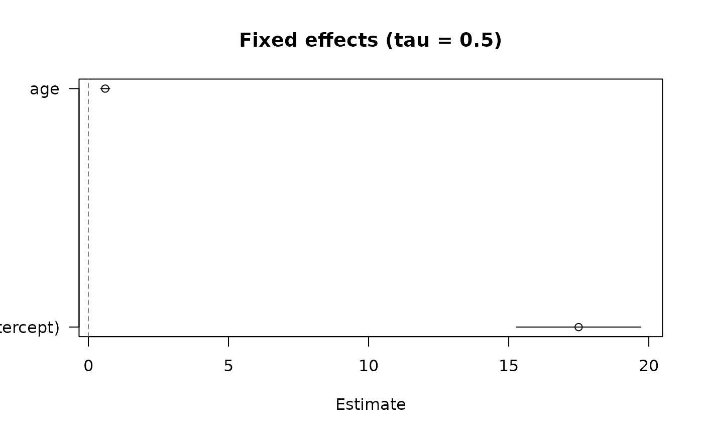
Default plot shows fixed-effect posterior intervals. With bayesplot
installed, richer MCMC plots are available via as_draws().
Usage
# S3 method for class 'bqmm'
plot(x, ...)Examples
# \donttest{
fit <- bqmm(distance ~ age + (1 | Subject), data = nlme::Orthodont,
tau = 0.5, chains = 1, iter = 300, refresh = 0, seed = 1)
#> Warning: The largest R-hat is 1.07, indicating chains have not mixed.
#> Running the chains for more iterations may help. See
#> https://mc-stan.org/misc/warnings.html#r-hat
#> Warning: Bulk Effective Samples Size (ESS) is too low, indicating posterior means and medians may be unreliable.
#> Running the chains for more iterations may help. See
#> https://mc-stan.org/misc/warnings.html#bulk-ess
#> Warning: Tail Effective Samples Size (ESS) is too low, indicating posterior variances and tail quantiles may be unreliable.
#> Running the chains for more iterations may help. See
#> https://mc-stan.org/misc/warnings.html#tail-ess
#> Warning: Some Rhat > 1.01; chains may not have converged.
#> Warning: Some effective sample sizes < 100; consider more iterations.
plot(fit)
 # }
# }