A Primer on Bayesian Multilevel Quantile Regression

Kailas Venkitasubramanian

This primer is written for applied researchers who have data, a question about how a predictor relates to the distribution of an outcome, and clustered or repeated measurements. It explains what Bayesian multilevel quantile regression is, when to reach for it, how to fit and interpret models with bqmm, and — just as important — how to check that the answer can be trusted. You do not need prior exposure to quantile regression or to Stan. Equations appear, but each is introduced in words first.

1. Why model quantiles?

Most regression you have met models the mean of an outcome: “on average, a one-unit change in x moves y by β.” That is often the wrong summary. Three situations recur in practice.

• The spread changes. In growth, income, or biomarker data the variability of the outcome grows with a predictor. A mean model reports one slope; the reality is that the 90th percentile rises far faster than the 10th.
• The tails are the point. Clinicians care about the patients at the high end of a risk marker, not the average patient; ecologists care about minimum river flow, not mean flow. These are questions about quantiles.
• The effect is distributional. A treatment may not shift everyone equally — it may compress the bottom of the distribution while leaving the top alone.

Quantile regression (Koenker 2005) answers these directly. Instead of the mean, it models a chosen conditional quantile — the median (τ = 0.5), the 10th percentile (τ = 0.1), the 90th (τ = 0.9), or a whole grid of them. The coefficient β(τ) is read as: “a one-unit change in x moves the τ-th percentile of y by β(τ).” Sweeping τ from 0 to 1 traces how a predictor reshapes the entire conditional distribution, not just its center.

Why multilevel?

Real data are rarely a single exchangeable sample. Patients are nested in hospitals; measurements are repeated within subjects; students are crossed with schools and neighbourhoods. Ignoring this structure understates uncertainty and discards information. Multilevel (mixed-effects) models add random effects — cluster-specific deviations drawn from a common distribution — so that each cluster borrows strength from the others while keeping its own signature.

Why Bayesian?

A Bayesian treatment delivers full posterior uncertainty for every quantity (fixed effects, variance components, predictions), handles the hierarchical shrinkage coherently, and lets you encode prior knowledge. It also comes with one subtlety specific to quantile regression — the likelihood is a working approximation — which Section 6 treats carefully. bqmm is built so that the default settings handle that subtlety for you.

2. The model in one page

Write the τ-th conditional quantile of the outcome for observation i in cluster j as a linear predictor with fixed and random parts:

$$Q_\tau(y_{ij} \mid x_{ij}, u_j) \;=\; x_{ij}^\top \beta(\tau) \;+\; z_{ij}^\top u_j .$$

Here β(τ) are the fixed effects at quantile τ (shared across clusters) and u_j are the random effects for cluster j, drawn from a mean-zero normal, u_j ~ N(0, Σ). The design vectors x and z are built from your formula — in bqmm you write y ~ x + (1 + x | g) exactly as in lme4.

The estimation trick. Classical quantile regression minimises the check loss ρ_τ(u) = u(τ − 1{u < 0}). There is no obvious likelihood to be Bayesian about — until you notice that minimising the check loss is equivalent to maximising the likelihood of the asymmetric Laplace distribution (ALD) (Yu and Moyeed 2001). So bqmm uses the ALD as a working likelihood:

$$y_{ij} \mid \cdot \;\sim\; \mathrm{ALD}\big(\mu_{ij},\, \sigma,\, \tau\big), \qquad \mu_{ij} = x_{ij}^\top\beta + z_{ij}^\top u_j ,$$

with a scale σ > 0. The mode/τ-quantile of this density sits exactly at the linear predictor, which is why fitting it recovers the quantile regression estimate. Priors complete the model: weakly-informative normals on β, half-normals on σ and the random-effect SDs, and (for correlated random effects) an LKJ prior on the correlation matrix. bqmm scales these defaults to your data so you rarely need to touch them.

Key idea. The ALD is a device, not a belief about your errors. It makes the quantile estimate computable in a Bayesian framework. Section 6 explains the one place this matters — uncertainty — and how bqmm corrects for it.

3. Your first model

We use the orthodontic growth data (nlme::Orthodont): the distance from the pituitary to the pterygomaxillary fissure, measured repeatedly on 27 children. Measurements are nested within Subject.

library(bqmm)
data(Orthodont, package = "nlme")

fit <- bqmm(distance ~ age + (1 | Subject),
            data = Orthodont,
            tau  = 0.5)          # the conditional median

summary(fit)

summary() reports the fixed effects with their Yang–Wang–He–adjusted intervals (Section 6), the random-effect standard deviations, and convergence notes. The familiar accessors all work:

fixef(fit)        # population-level coefficients at tau = 0.5
ranef(fit)        # subject-specific deviations
VarCorr(fit)      # random-effect SDs (and correlations, if any)
coef(fit)         # fixed effects
predict(fit)      # fitted conditional medians

4. Many quantiles at once

The power of quantile regression is comparison across τ. Pass a vector:

fit_q <- bqmm(distance ~ age + (1 | Subject),
              data = Orthodont,
              tau  = c(0.1, 0.25, 0.5, 0.75, 0.9))

coef(fit_q)   # a tau-by-coefficient matrix
plot(fit_q)   # coefficient-versus-tau paths

The coefficient path shows how the age effect changes across the distribution of growth. If the slope rises with τ, older children’s upper percentiles grow faster than their lower ones — a fanning-out the mean model cannot express.

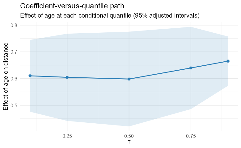
Coefficient-versus-quantile path: the estimated effect of a predictor at each quantile, with uncertainty. A non-flat path is distributional information a mean model discards.

Non-crossing. Fitted quantile curves estimated separately can cross, which is logically impossible (the 10th percentile cannot exceed the 90th). bqmm offers a post-hoc fix — sorting the fitted values across τ (Chernozhukov et al. 2010):

predict(fit_q, noncrossing = "rearrange")

5. Priors and the scale parameter

The defaults are weakly informative and scaled to your response, chosen to keep the sampler stable rather than to inject information. Override any of them with bqmm_prior():

my_prior <- bqmm_prior(
  beta_sd     = 5,    # SD of the normal prior on fixed effects
  sigma_scale = 1,    # half-normal scale for the ALD scale sigma
  re_scale    = 2,    # half-normal scale for random-effect SDs
  lkj         = 2     # LKJ shape (correlated REs only)
)
fit <- bqmm(distance ~ age + (1 | Subject), Orthodont,
            tau = 0.5, prior = my_prior)

The ALD scale σ is a nuisance parameter of the working likelihood. It governs the spread of the working density but is not the residual SD of your data, and you should not interpret it as such. Its main job is to be marginalised over; bqmm’s inference correction (next) removes any dependence of the reported uncertainty on the precise value of σ.

6. Getting the uncertainty right

This is the most important section. Because the ALD is a working likelihood, the naive Bayesian posterior covariance of the fixed effects is not the correct sampling variance of the quantile-regression estimator — credible intervals built from it can badly under- or over-cover (Yang et al. 2016). This is a known, well-understood issue, and bqmm corrects for it by default.

The correction follows Yang et al. (2016): replace the naive posterior covariance with a sandwich that re-uses the posterior covariance as its “bread” and a score-variance “meat”,

$$V_{\mathrm{adj}} \;=\; \Sigma_{\text{post}}\; G\; \Sigma_{\text{post}},$$

where G is the variance of the ALD working-likelihood score. Using the posterior covariance as the bread is what makes this valid for multilevel models: Σ_post already carries the random-effect contribution to fixed-effect uncertainty, so the correction keeps it while fixing the misspecified scale. Under correct specification the correction collapses to ≈ Σ_post, as it should.

vcov(fit, adjusted = TRUE)    # corrected (default)
vcov(fit, adjusted = FALSE)   # naive posterior covariance
confint(fit, adjusted = TRUE)
summary(fit)                  # uses the adjusted intervals

In simulation across homoscedastic and heteroscedastic two-level designs, the adjusted intervals cover at or just above the nominal 95%, whereas the naive intervals under-cover the slopes; see vignette("bqmm-inference") and the package’s review report. The take-away for practice:

Report adjusted = TRUE intervals unless you have a specific reason not to. They are the package’s reason to exist over a generic ALD fit.

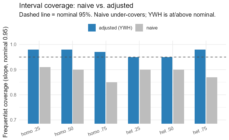
Frequentist coverage of nominal-95% intervals across simulated designs: the naive posterior under-covers; the Yang–Wang–He–adjusted intervals are at or above nominal.

7. Correlated random effects

A random intercept and slope are usually correlated — children who start tall may also grow faster. Model that correlation with cov = "unstructured":

fit_c <- bqmm(distance ~ age + (1 + age | Subject),
              data = Orthodont, tau = 0.5,
              cov  = "unstructured")

VarCorr(fit_c)                       # SDs plus...
attr(VarCorr(fit_c), "correlation")  # the posterior-median correlation matrix

An LKJ prior (default shape 2, mildly favouring weak correlation) regularises the correlation. Two cautions:

• The covariance is only weakly identified when the random effects are small relative to the noise, or when there are few clusters. If the estimated SDs or correlation look shrunk toward zero, you likely lack the information to estimate them — not a bug. Prefer many clusters.
• cov = "unstructured" currently supports a single grouping factor. For multiple or crossed terms, use cov = "diagonal" (the default).

8. Diagnostics: is the fit trustworthy?

A posterior you cannot trust is worse than no posterior. Always check:

Sampler convergence. bqmm surfaces warnings automatically — split-R̂ above 1.01, low effective sample size, or divergent transitions. Treat any of these as a stop sign. The usual fixes:

fit <- bqmm(distance ~ age + (1 | Subject), Orthodont, tau = 0.5,
            chains = 4, iter = 4000,
            control = list(adapt_delta = 0.99, max_treedepth = 12))

Raising adapt_delta toward 0.99 and increasing iter cures most divergences and low-ESS warnings; variance and correlation parameters are the slowest to mix and benefit most. Inspect them with the posterior and bayesplot ecosystems:

library(posterior)
summarise_draws(as_draws(fit))            # R-hat, ESS per parameter

library(bayesplot)
mcmc_trace(as_draws(fit), regex_pars = "b_")

Posterior predictive checks. Does the fitted model generate data that look like yours? Overlay replicated datasets on the observed outcome:

yrep <- posterior_predict(fit)            # draws x observations
bayesplot::ppc_dens_overlay(Orthodont$distance, yrep[1:50, ])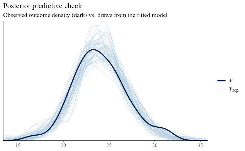

Posterior predictive check: the observed outcome density (dark) against draws from the fitted model (light). Systematic mismatch flags a misfit the quantile of interest may not capture.

Non-crossing. When fitting several τ, confirm the fitted quantiles are monotone (or enforce it with noncrossing = "rearrange").

9. Visualising results

Three plots carry most of the message:

1. Coefficient-versus-τ paths (plot() on a multi-quantile fit) — the headline distributional story.
2. Fitted quantile curves over a predictor grid, optionally rearranged, to show the conditional distribution fanning across the data.
3. Posterior predictive overlays (ppc_dens_overlay) and parameter intervals (bayesplot::mcmc_areas(as_draws(fit))) for fit and uncertainty.

Because as_draws() exposes the fit to the whole posterior/bayesplot stack, any plot in those packages is available with tidy parameter names (b_<coef>, sd_<component>, sigma).

10. Practical guidance and pitfalls

• Clusters, not just observations. Random-effect variances and correlations need many groups (rule of thumb: ≥ 20–30) to be estimable. A handful of large clusters is not enough.
• Extreme quantiles need more data. τ = 0.05 or 0.95 are estimated from the sparse tail; expect wider intervals and harder sampling. Raise adapt_delta.
• Scale your predictors. Centring and scaling continuous predictors improves sampling geometry and makes priors easier to set.
• Diagonal vs unstructured. Start with cov = "diagonal". Move to "unstructured" only when you have one grouping factor, enough clusters, and a substantive reason to expect correlated random effects.
• cores > 1 parallelises chains; on some systems the package must be on the default library path for the parallel workers to find it. cores = 1 always works.
• Report the quantile(s) modelled, the adjusted intervals, the random-effect SDs (and correlations), and your convergence diagnostics.

11. How bqmm relates to other tools

• lqmm, qrLMM — frequentist quantile mixed models; excellent point estimation, no posterior. bqmm’s fixed-effect estimates agree closely with lqmm.
• brms (asym_laplace) — can fit a multilevel ALD model, but with a fixed quantile, an awkward scale, and uncorrected (invalid) intervals. bqmm’s reason to exist is the corrected inference and a quantile-first interface.
• bayesQR, Brq — Bayesian quantile regression without random effects.

References

Chernozhukov, Victor, Iván Fernández-Val, and Alfred Galichon. 2010. “Quantile and Probability Curves Without Crossing.” Econometrica 78 (3): 1093–125.

Koenker, Roger. 2005. Quantile Regression. Econometric Society Monographs. Cambridge University Press.

Yang, Yunwen, Huixia Judy Wang, and Xuming He. 2016. “Posterior Inference in Bayesian Quantile Regression with Asymmetric Laplace Likelihood.” International Statistical Review 84 (3): 327–44.

Yu, Keming, and Rana A. Moyeed. 2001. “Bayesian Quantile Regression.” Statistics & Probability Letters 54 (3): 437–47.